So much more than pretty graphs
The value of creating and implementing a dataviz design system in R
NHSR 2023 | 11th October 2023
Hi there 👋 !
Just in case…

@cararthompson

Hi there 👋 !
Just in case…

@cararthompson
Hi there 👋 !
Dataviz Design System, implemented as an R package
Hi there 👋 !
Dataviz Design System, implemented as an R package
Gathering specific requirements
- What kind of colours would you like to be associated with this project?
- How many colours do you need?
- Any colour semantics we should include?

- What types of plots do you use a lot?
- How much personality would you like to convey in the text formatting?
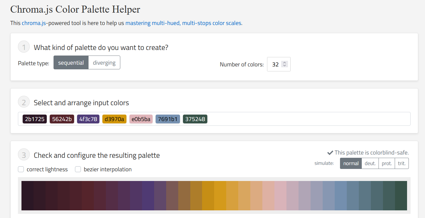
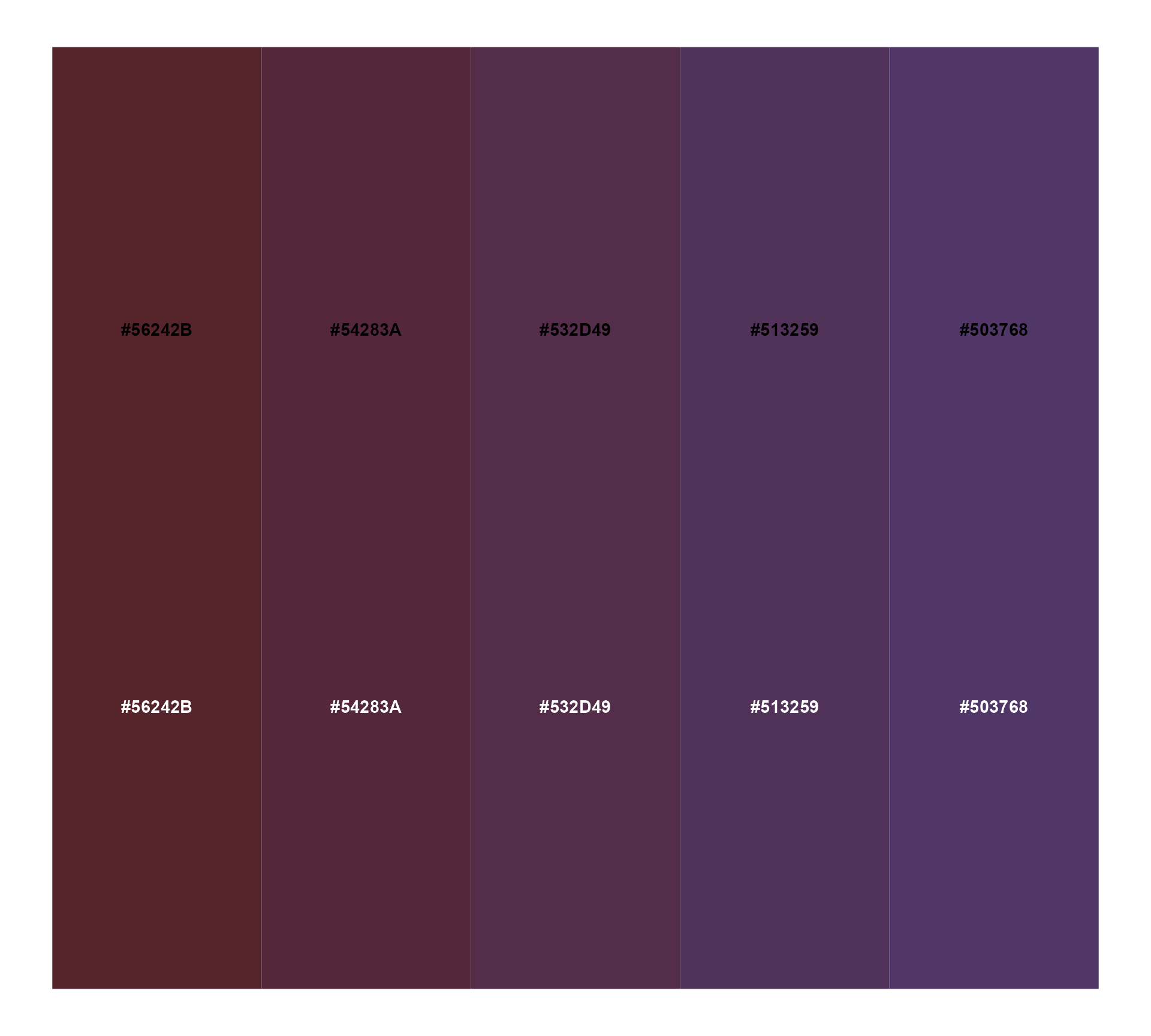
Colour inspiration
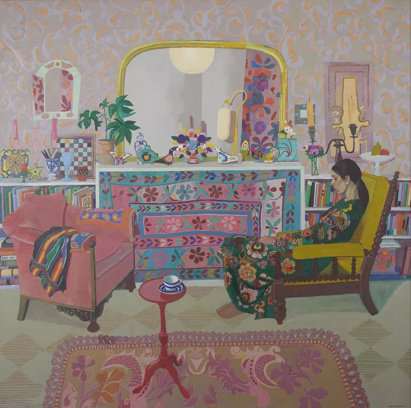
Colour inspiration
Colour inspiration 🥳
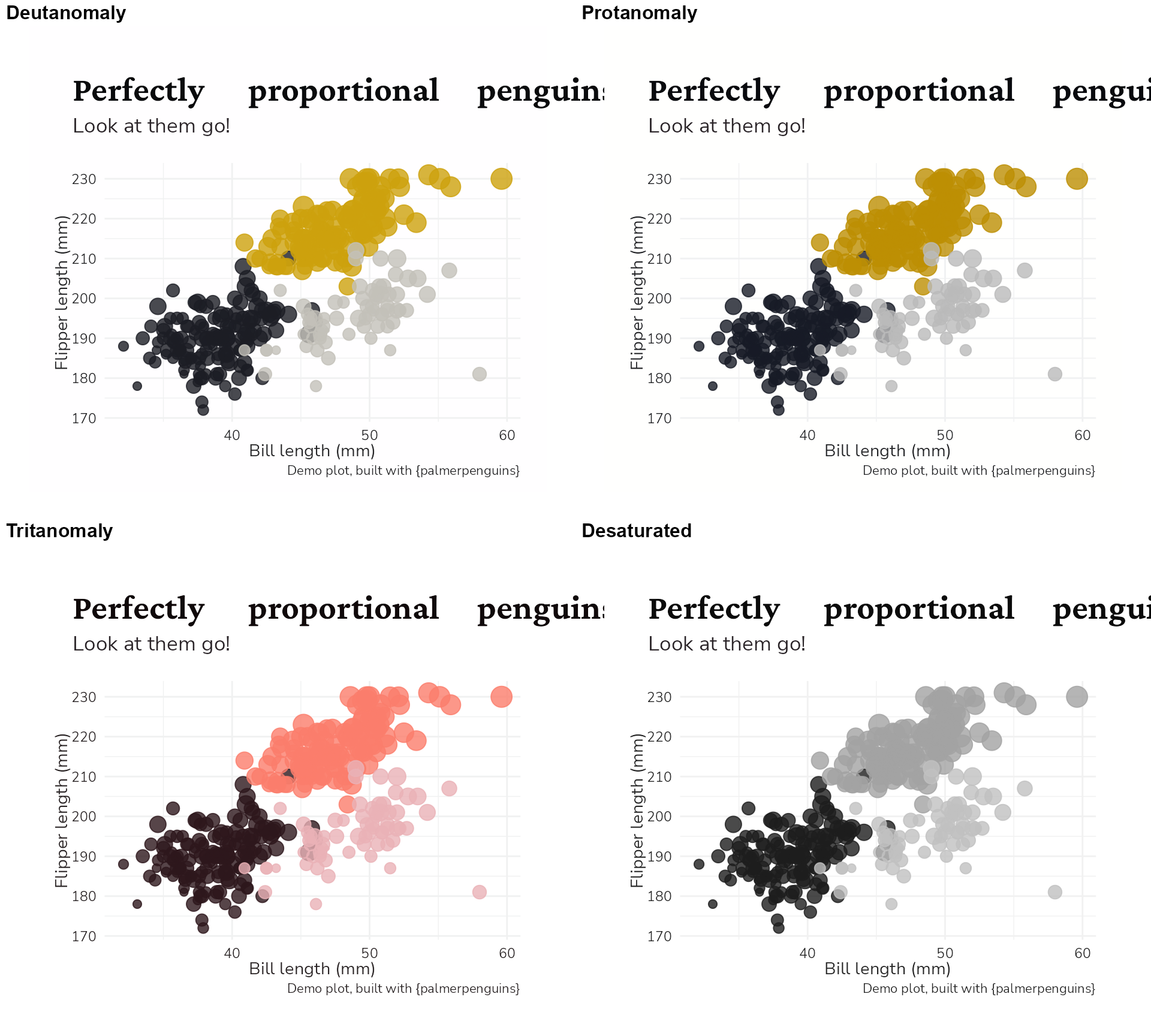
Colours & Accessibility
More than green and red!
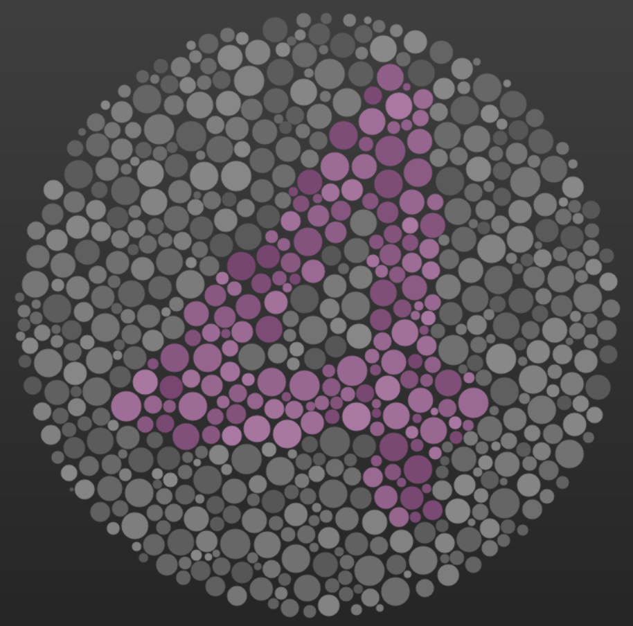
- Colour perception differences
- Green / Red / Blue / Combinations
- Neurodivergent audiences - 10-15% of global population
- Behavioural / emotional disorders
- ADHD
- Learning disabilities
- Autism
Colours & Accessibility
Top tips
- Shades of the same colour rather than lots of different colours
- Prefer muted colours over stark contrasts
- Less is more
- Light/dark variation as well as hue variation
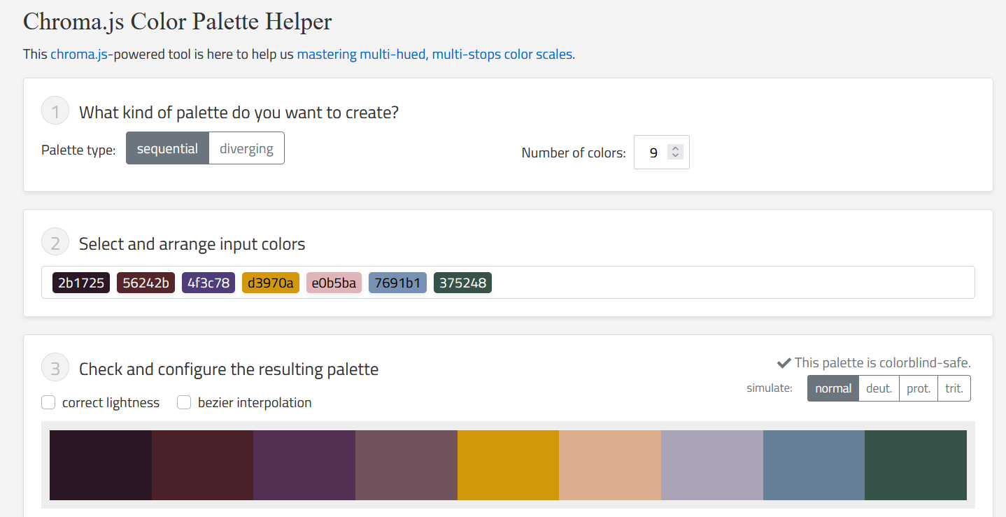
Colours & Accessibility
R: {monochromeR} + {colorblindr}
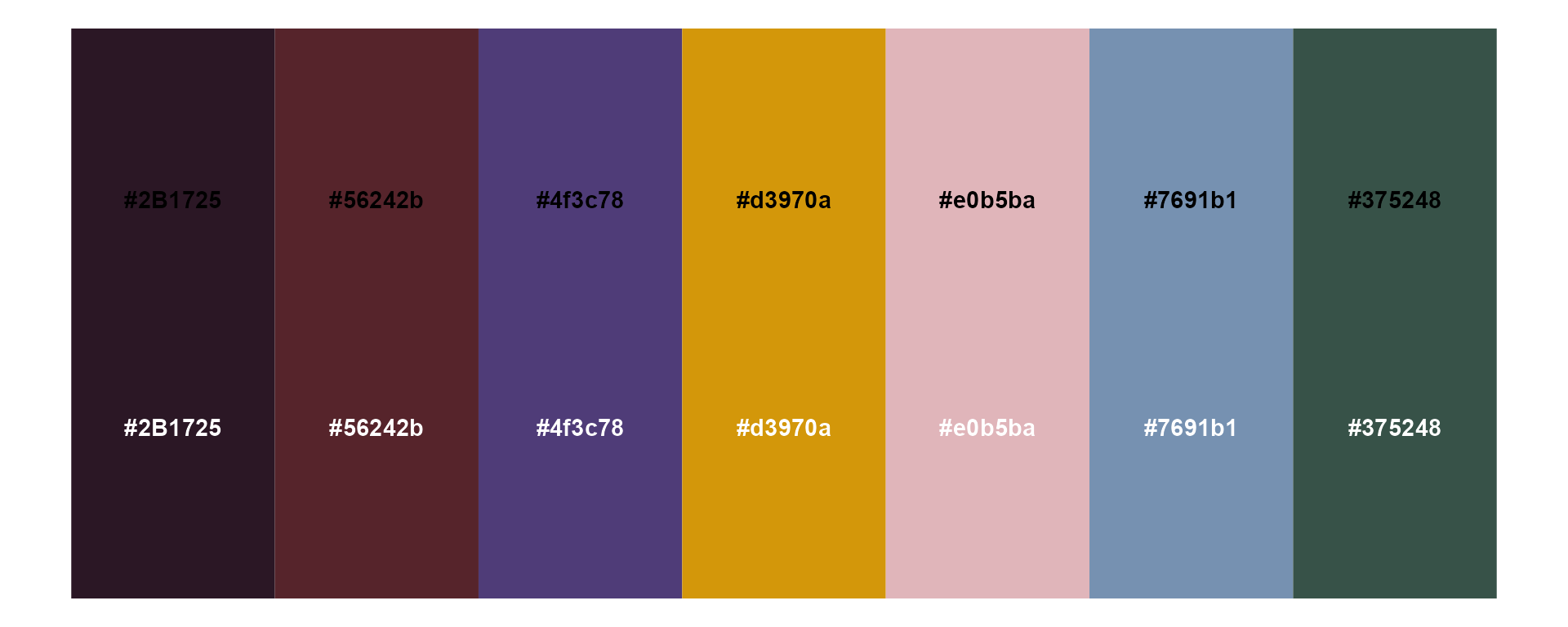
Colours & Accessibility
R: {monochromeR} + {colorblindr}
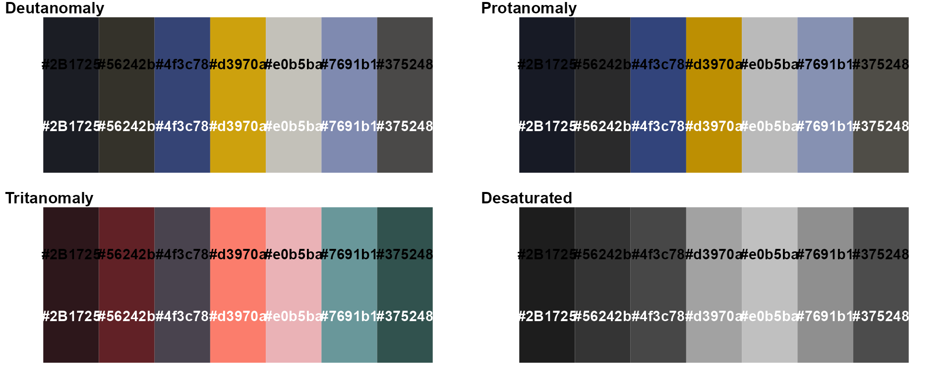
Colours & Accessibility
R: {monochromeR} + {colorblindr}
library(tidyverse)
palmerpenguins::penguins |>
ggplot() +
geom_point(aes(x = bill_length_mm,
y = flipper_length_mm,
size = body_mass_g,
color = species),
alpha = 0.8) +
labs(title = "Perfectly proportional penguins",
subtitle = "Look at them go!",
x = "Bill length (mm)",
y = "Flipper length (mm)",
caption = "Demo plot, built with {palmerpenguins}") +
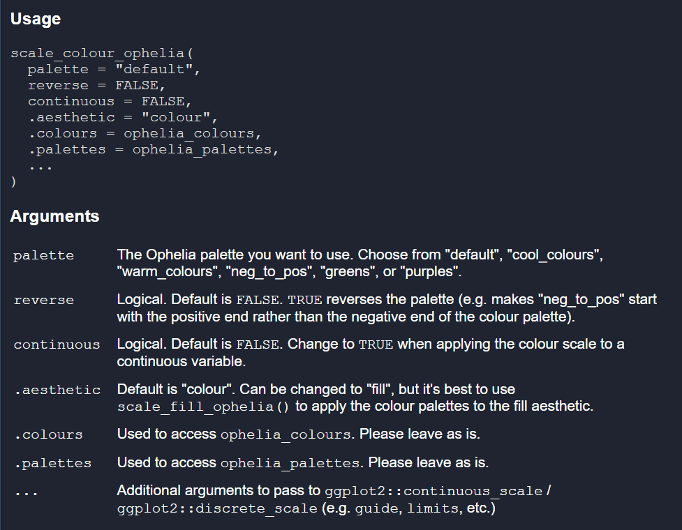
ophelia::scale_colour_ophelia(palette = "warm_colours",
continuous = FALSE) +
ophelia::theme_ophelia(background = FALSE) +
theme(legend.position = "none")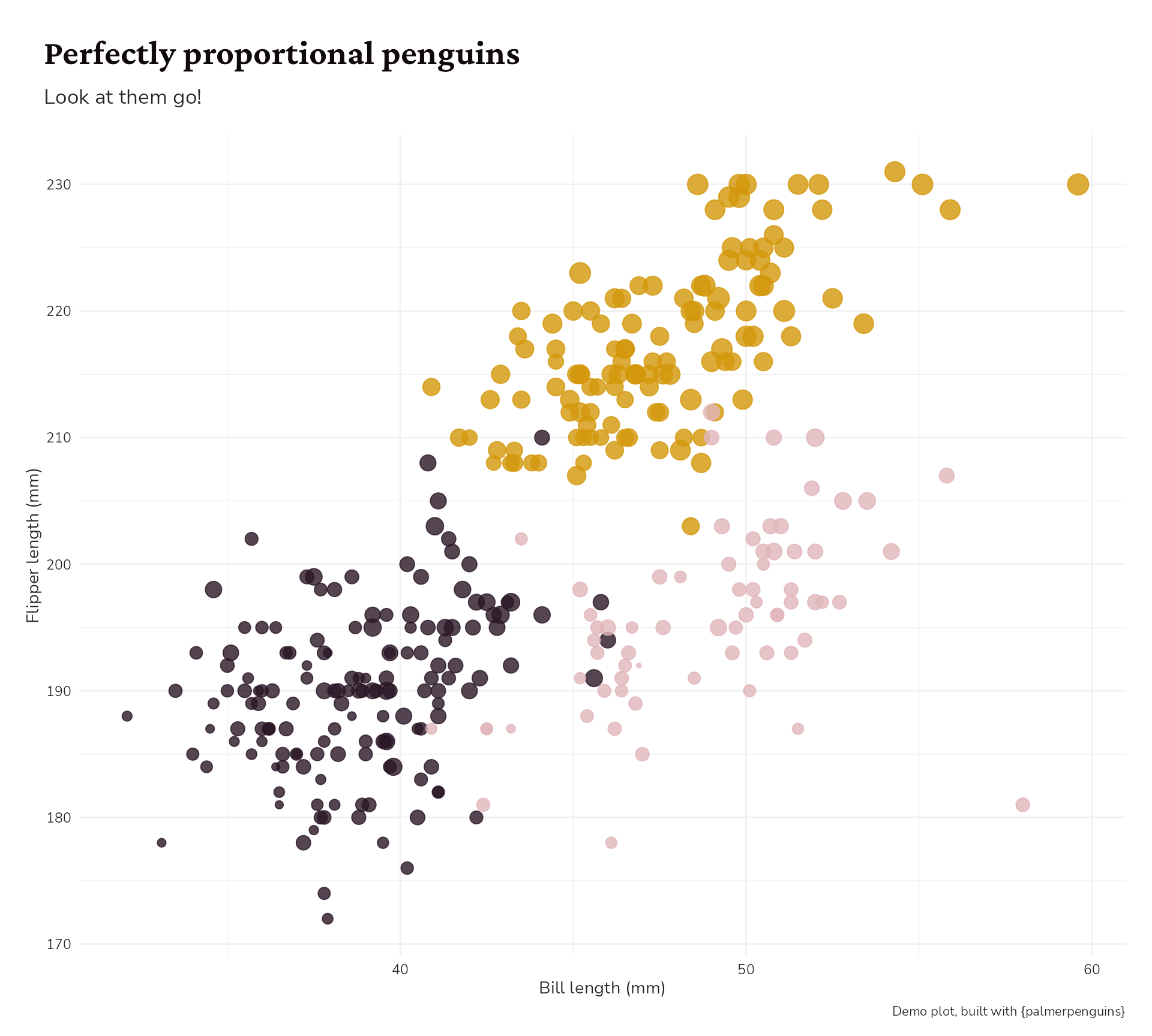
Colours & Accessibility
R: {monochromeR} + {colorblindr}
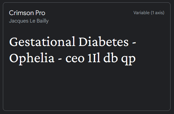
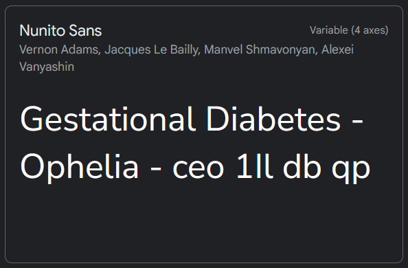
Font inspiration
- Make it easy for the end user!
- Easy to find & install
.ttf- Italics & bold
- Numbers & special characters
- Easy to read
Font inspiration
- Make it easy for the end user!
- Easy to find & install
.ttf- Italics & bold
- Numbers & special characters
- Easy to read
Fonts & usability
Getting custom fonts to work can be frustrating!
Install fonts locally, restart R Studio + 📦
{systemfonts}({ragg}+{textshaping}) + Set graphics device to “AGG” + 🤞
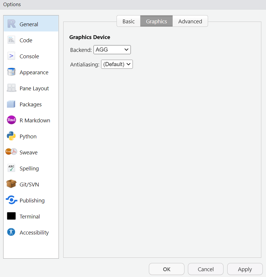
knitr::opts_chunk$set(dev = “ragg_png”)

Colours
… with a few extra touches
Colours
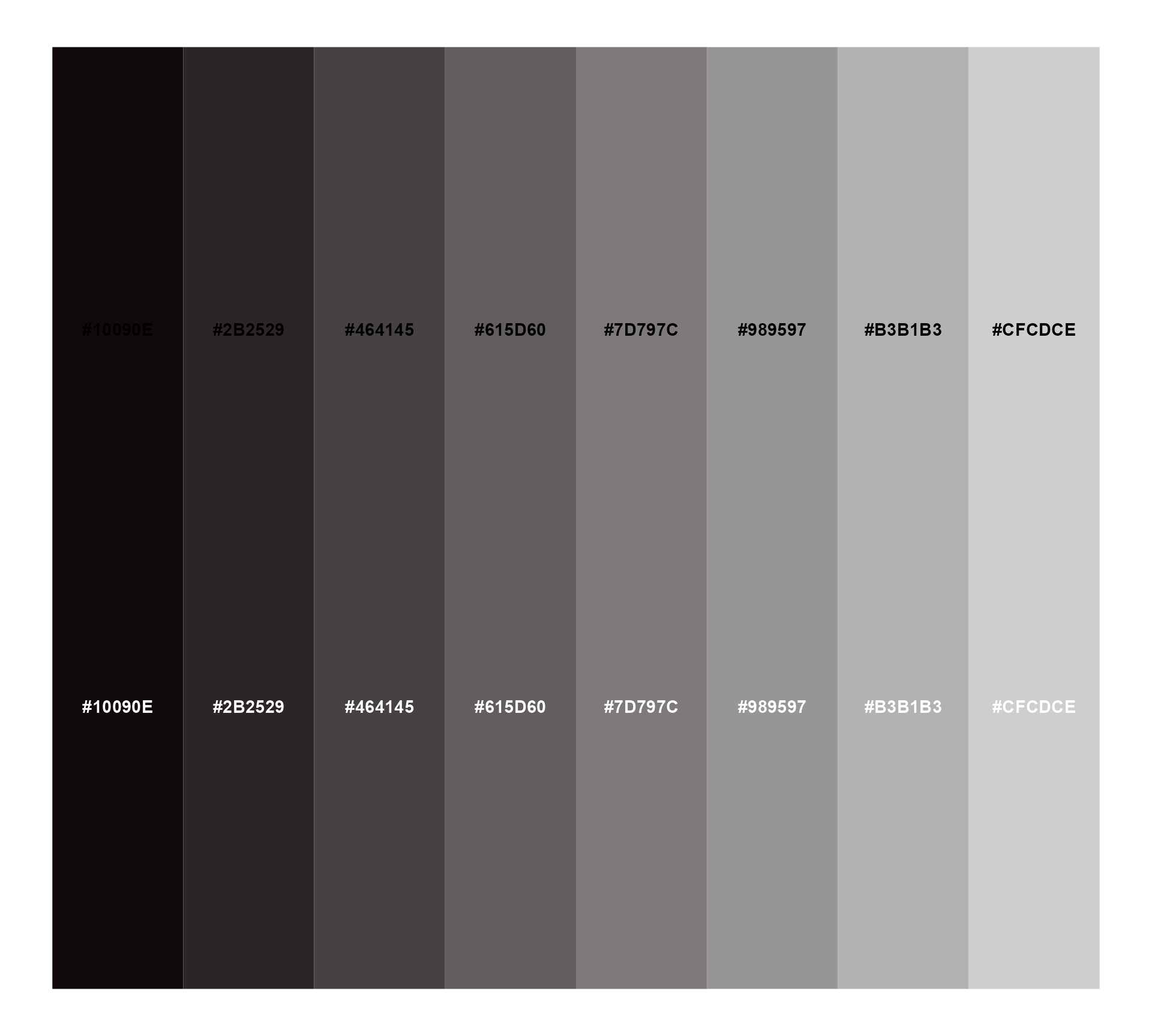
Text colours: find a “starting” colour the ties in with all the palettes
Colours
Text colours: feed it into {monochromeR} to generate a dark text colour
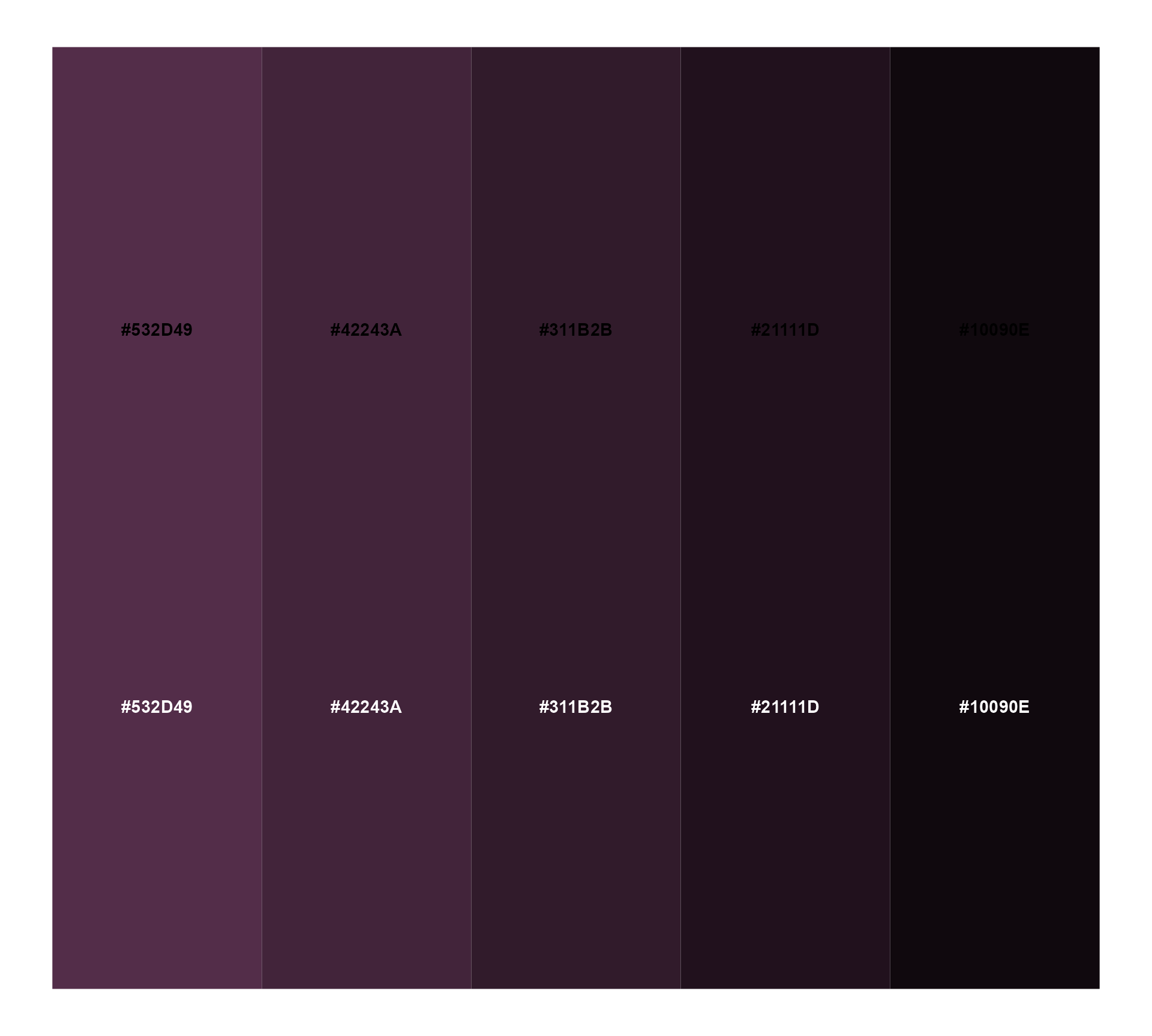
Colours
Text colours: feed that dark text colour into {monochromeR} again to generate a light text colour
Plot theme
… with a few option toggles
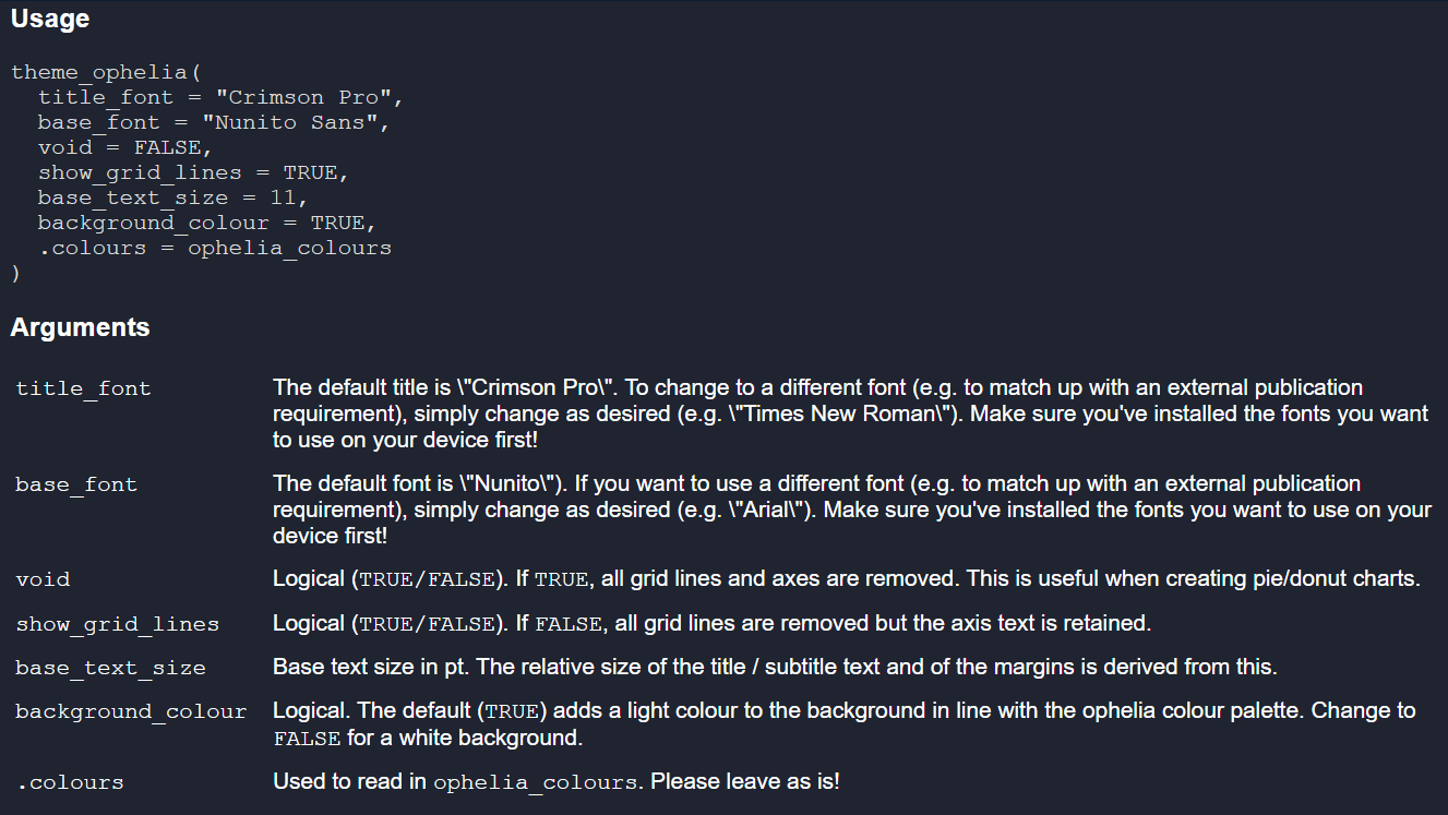
Two extra lines
palmerpenguins::penguins %>%
ggplot() +
geom_point(aes(x = bill_length_mm,
y = flipper_length_mm,
colour = species,
size = body_mass_g)) +
labs(x = "Bill length (mm)",
y = "Flipper length (mm)",
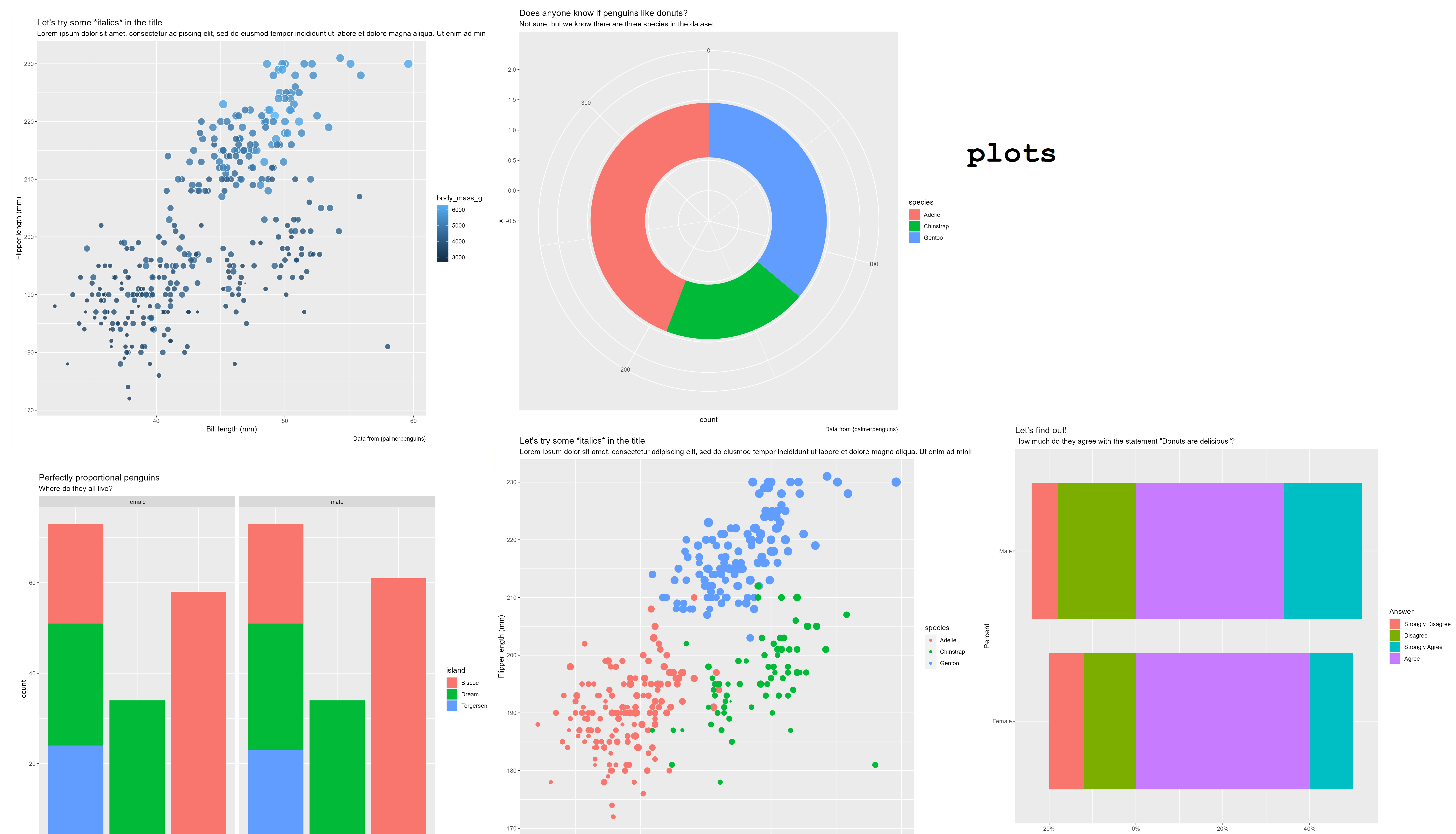
title = "Let's try some *italics* in the title",
subtitle = "Lorem ipsum dolor sit amet, consectetur adipiscing elit, sed do eiusmod tempor incididunt ut labore et dolore magna aliqua. Ut enim ad minim veniam, quis nostrud exercitation ullamco laboris nisi ut aliquip ex ea commodo consequat.",
caption = "Data from {palmerpenguins}") +
guides(size = "none")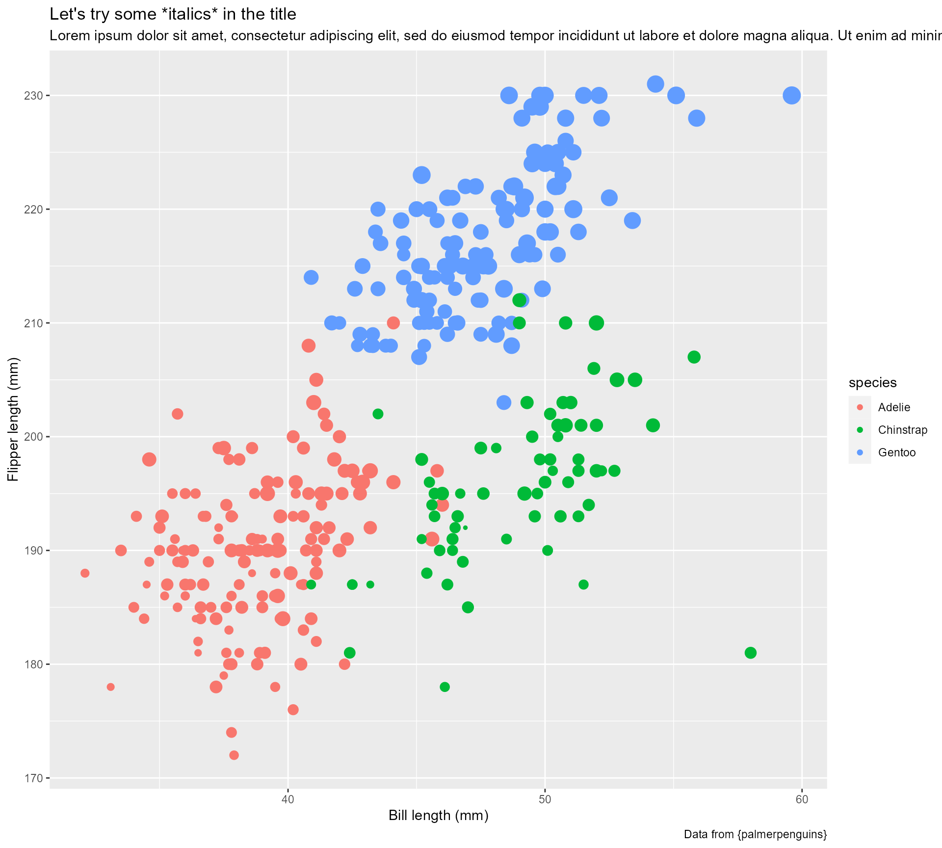
Two extra lines
palmerpenguins::penguins %>%
ggplot() +
geom_point(aes(x = bill_length_mm,
y = flipper_length_mm,
colour = species,
size = body_mass_g)) +
labs(x = "Bill length (mm)",
y = "Flipper length (mm)",
title = "Let's try some *italics* in the title",
subtitle = "Lorem ipsum dolor sit amet, consectetur adipiscing elit, sed do eiusmod tempor incididunt ut labore et dolore magna aliqua. Ut enim ad minim veniam, quis nostrud exercitation ullamco laboris nisi ut aliquip ex ea commodo consequat.",
caption = "Data from {palmerpenguins}") +
guides(size = "none") +
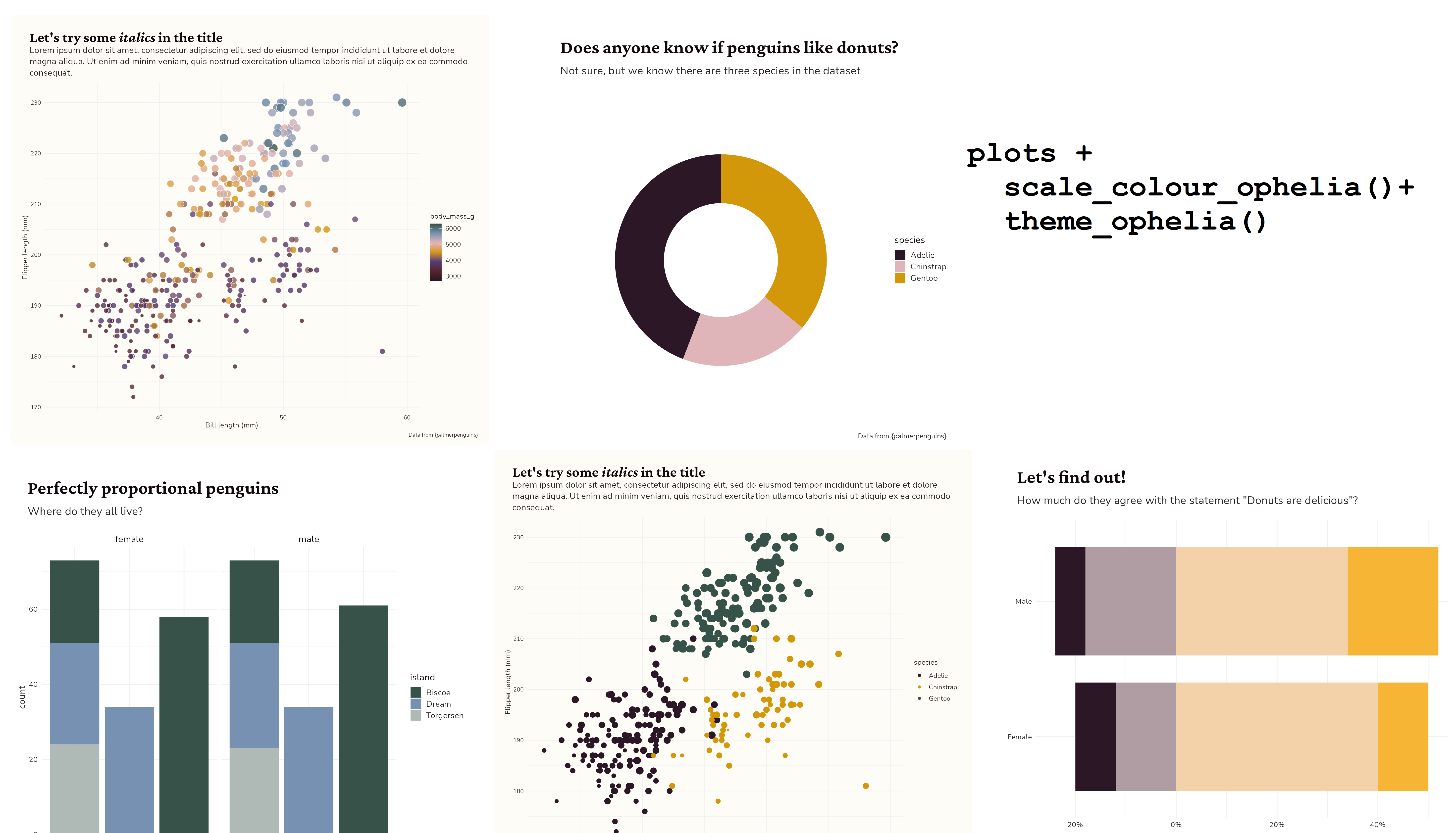
scale_colour_ophelia() +
theme_ophelia()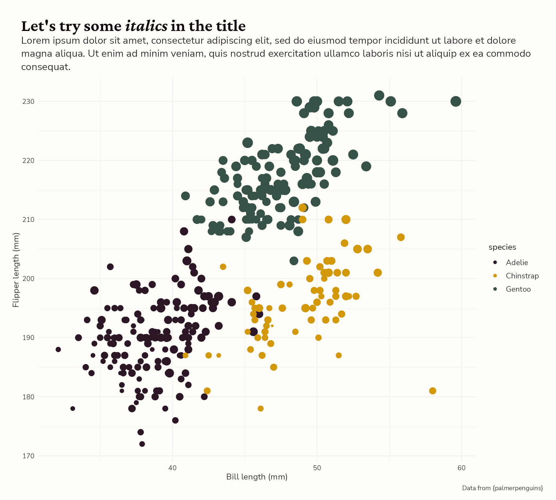
Two extra lines
palmerpenguins::penguins %>%
  ggplot() +
  geom_point(aes(x = bill_length_mm,
                 y = flipper_length_mm,
                 fill = body_mass_g,
                 size = body_mass_g),
             shape = 21,
             colour = "white",
             alpha = 0.8) +
  labs(x = "Bill length (mm)",
       y = "Flipper length (mm)",
       title = "Let's try some *italics* in the title",
       subtitle = "Lorem ipsum dolor sit amet, consectetur adipiscing elit, sed do eiusmod tempor incididunt ut labore et dolore magna aliqua. Ut enim ad minim veniam, quis nostrud exercitation ullamco laboris nisi ut aliquip ex ea commodo consequat.",
       caption = "Data from {palmerpenguins}") +
  guides(size = "none")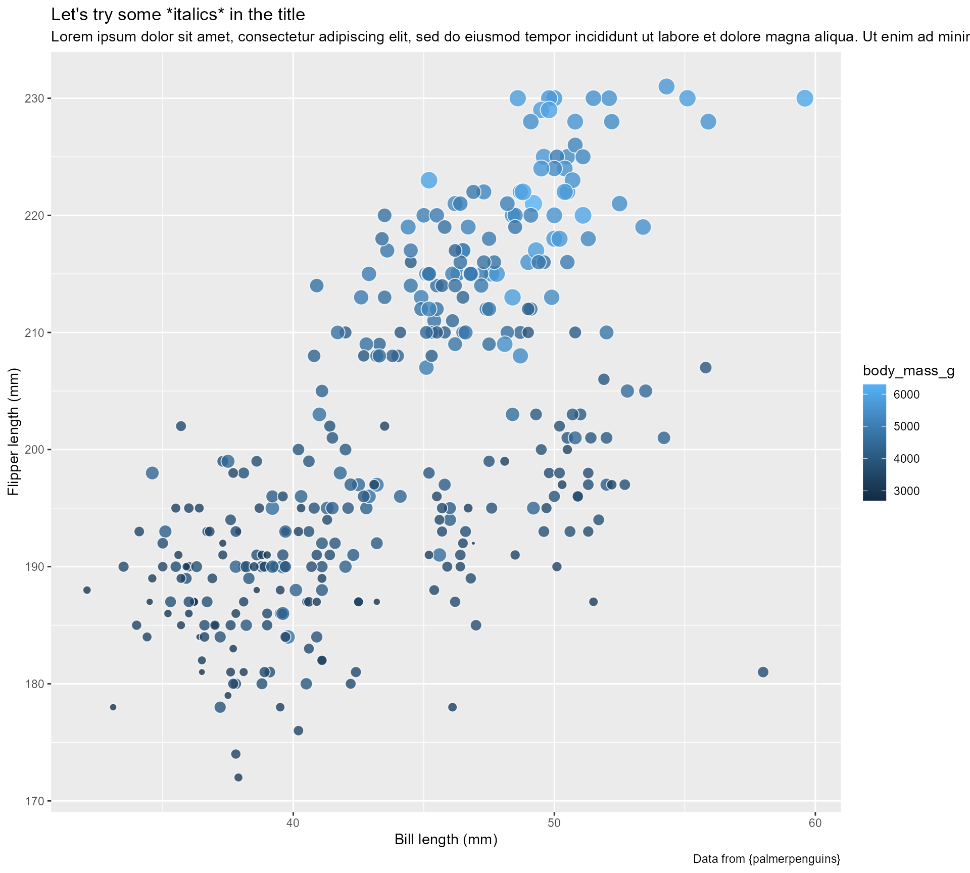
Two extra lines
palmerpenguins::penguins %>%
  ggplot() +
  geom_point(aes(x = bill_length_mm,
                 y = flipper_length_mm,
                 fill = body_mass_g,
                 size = body_mass_g),
             shape = 21,
             colour = "white",
             alpha = 0.8) +
  labs(x = "Bill length (mm)",
       y = "Flipper length (mm)",
       title = "Let's try some *italics* in the title",
       subtitle = "Lorem ipsum dolor sit amet, consectetur adipiscing elit, sed do eiusmod tempor incididunt ut labore et dolore magna aliqua. Ut enim ad minim veniam, quis nostrud exercitation ullamco laboris nisi ut aliquip ex ea commodo consequat.",
       caption = "Data from {palmerpenguins}") +
  guides(size = "none") +
  scale_fill_ophelia(continuous = TRUE) +
  theme_ophelia()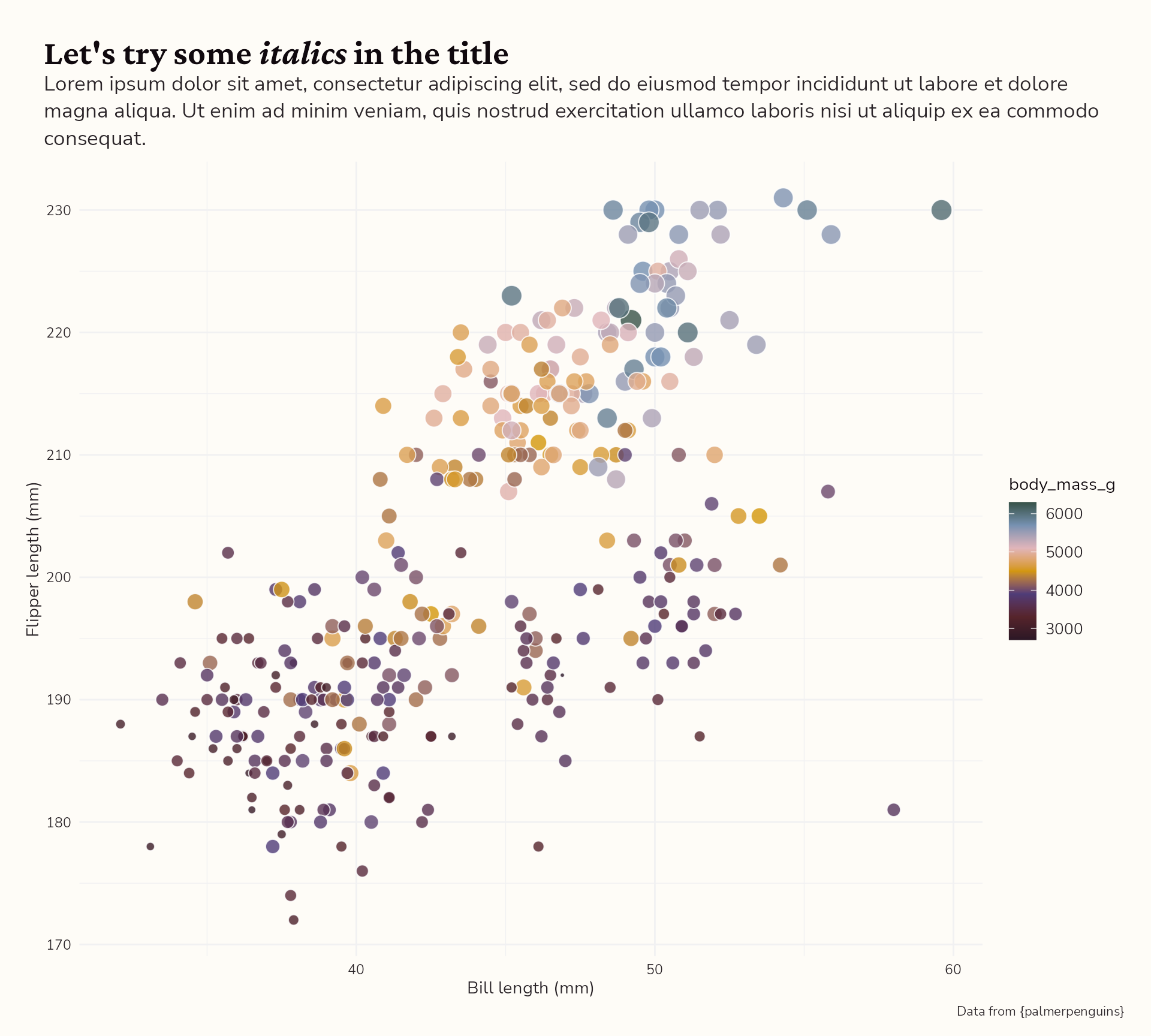
Two extra lines
palmerpenguins::penguins %>%
  ggplot() +
  geom_point(aes(x = bill_length_mm,
                 y = flipper_length_mm,
                 fill = body_mass_g,
                 size = body_mass_g),
             shape = 21,
             colour = "white",
             alpha = 0.8) +
  labs(x = "Bill length (mm)",
       y = "Flipper length (mm)",
       title = "Let's try some *italics* in the title",
       subtitle = "Lorem ipsum dolor sit amet, consectetur adipiscing elit, sed do eiusmod tempor incididunt ut labore et dolore magna aliqua. Ut enim ad minim veniam, quis nostrud exercitation ullamco laboris nisi ut aliquip ex ea commodo consequat.",
       caption = "Data from {palmerpenguins}") +
  guides(size = "none") +
  scale_fill_ophelia(continuous = TRUE) +
  theme_ophelia(base_text_size = 18)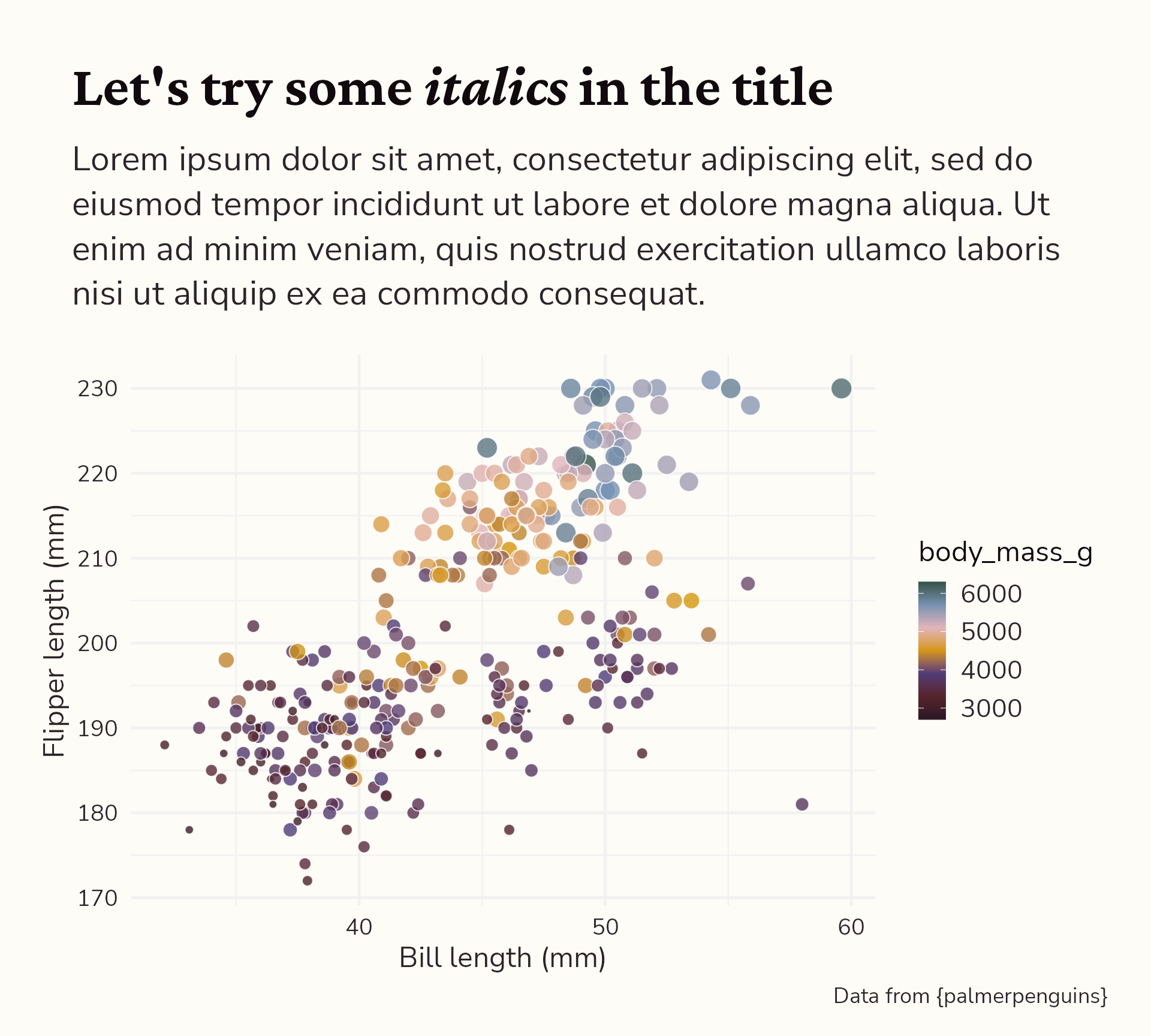
Two extra lines
Two extra lines
palmerpenguins::penguins %>%
filter(!is.na(sex)) %>%
ggplot(aes(x = species,
fill = island),
stat = "count") +
geom_bar() +
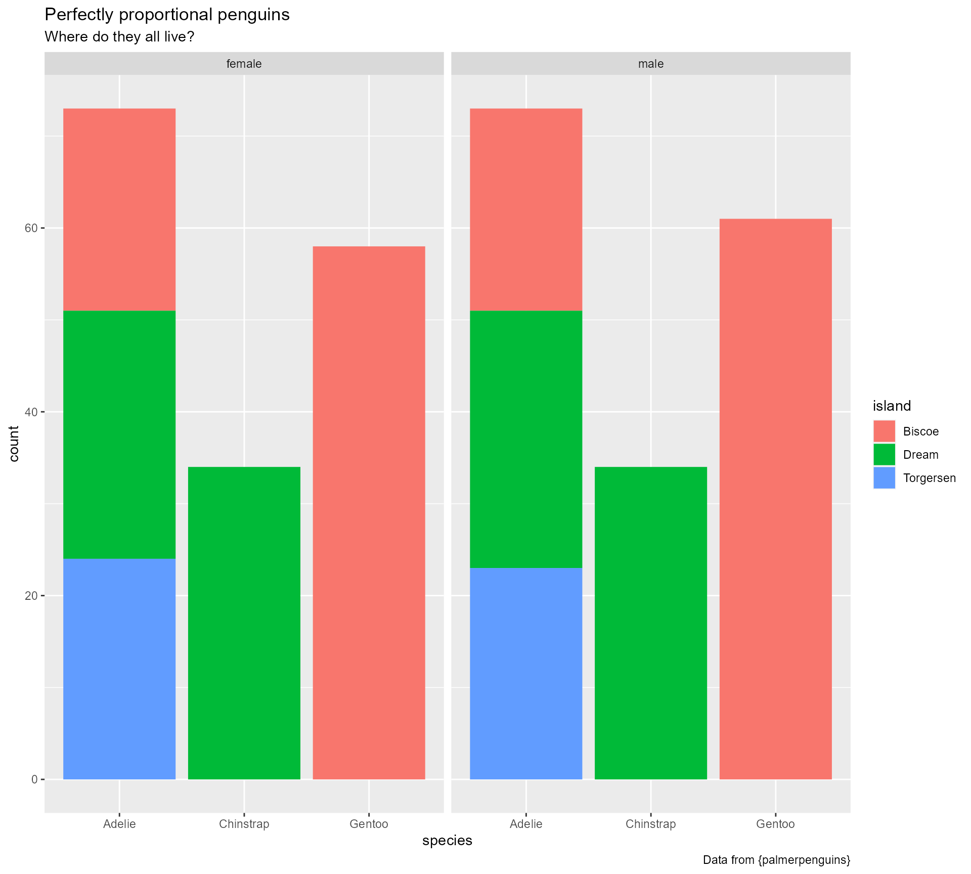
labs(title = "Perfectly proportional penguins",
subtitle = "Where do they all live?",
caption = "Data from {palmerpenguins}") +
facet_grid(. ~ sex) +
scale_fill_ophelia(palette = "cool_colours") +
theme_ophelia(background_colour = FALSE,
base_text_size = 14)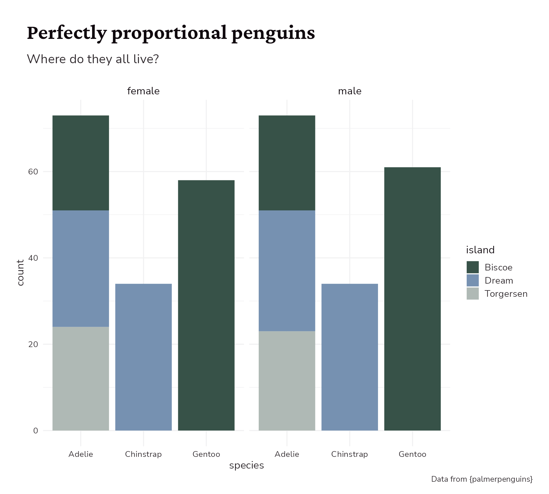
Two extra lines
palmerpenguins::penguins %>%
  ggplot(aes(x = 1,
             fill = species),
         stat = "count") +
  geom_bar() +
  xlim(c(-0.5, 2)) +
  coord_polar(theta = "y") +
  labs(title = "Does anyone know if penguins like donuts?",
       subtitle = "Not sure, but we know there are three species in the dataset",
       caption = "Data from {palmerpenguins}")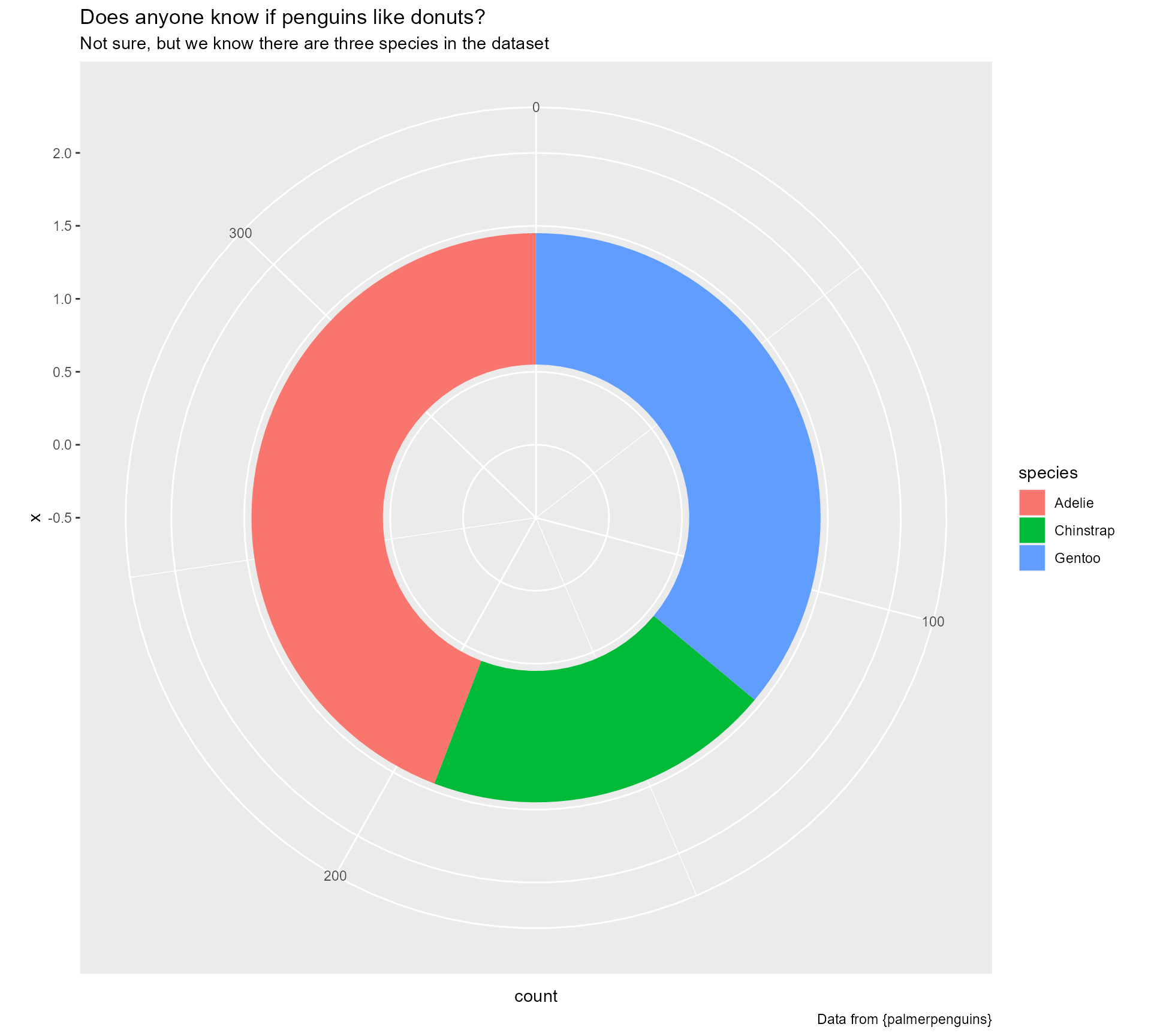
Two extra lines
palmerpenguins::penguins %>%
  ggplot(aes(x = 1,
             fill = species),
         stat = "count") +
  geom_bar() +
  xlim(c(-0.5, 2)) +
  coord_polar(theta = "y") +
  labs(title = "Does anyone know if penguins like donuts?",
       subtitle = "Not sure, but we know there are three species in the dataset",
       caption = "Data from {palmerpenguins}") +
  scale_fill_ophelia("warm_colours") +
  theme_ophelia(void = TRUE,
                base_text_size = 14,
                background_colour = FALSE)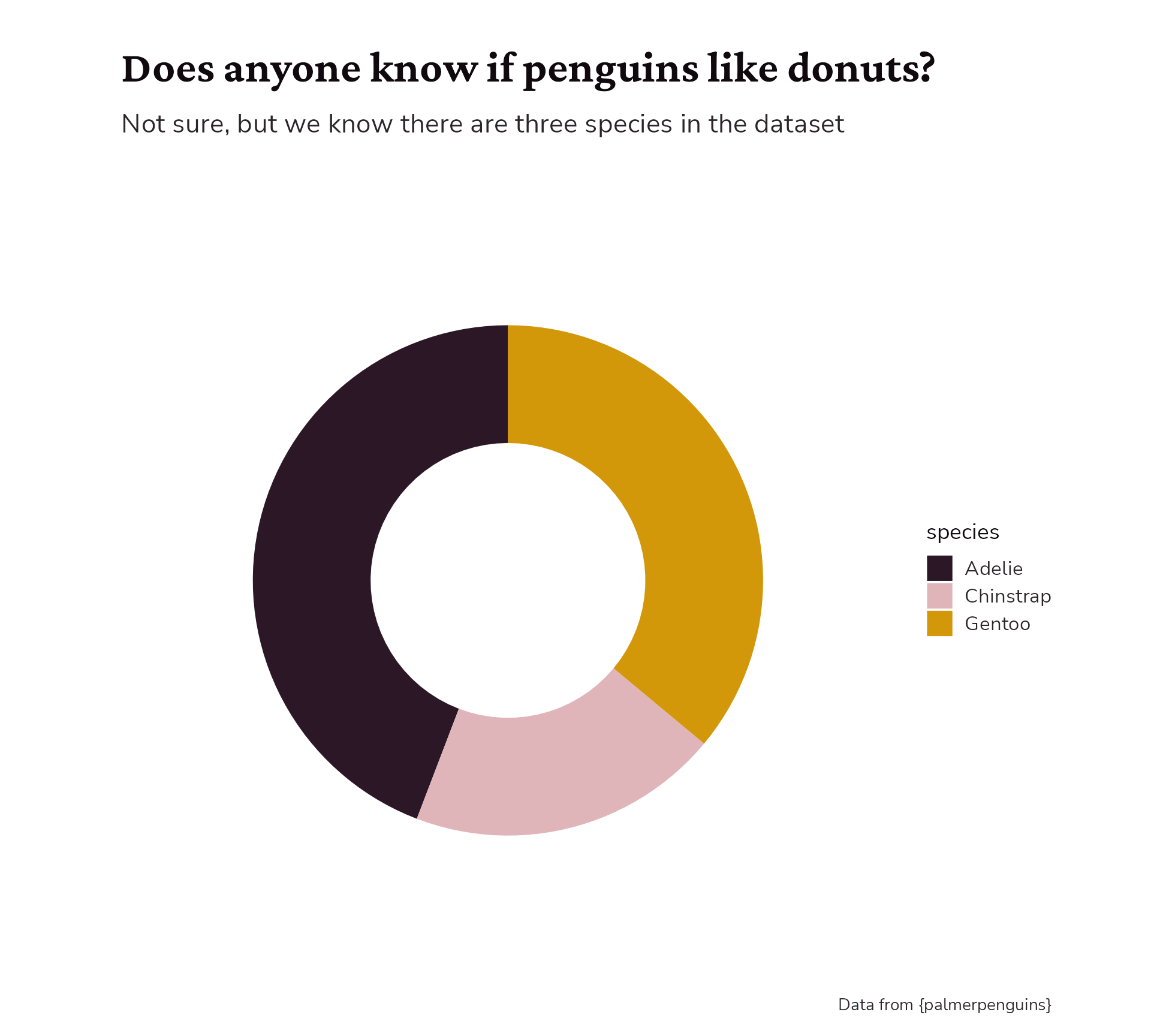
Two extra lines
tibble(answer = factor(rep(c("Strongly Disagree", "Disagree",
                             "Agree", "Strongly Agree"), 2),
                       levels = c("Strongly Disagree", "Disagree",
                                  "Strongly Agree", "Agree")),
       percent = c(8, 12, 40, 10,
                   6, 18, 34, 18),
       group = sort(rep(c("Male", "Female"), 4))) %>%
  mutate(display_percent = case_when(grepl("Dis|Neutral", answer) ~ -percent,
                                     TRUE ~ percent)) %>%
  ggplot() +
  geom_col(aes(x = group,
               fill = answer,
               y = display_percent),
           width = 0.8) +
  labs(title = "Let's find out!",
       subtitle = "How much do they agree with the statement \"Donuts are delicious\"?",
       caption = "Totally made up data!",
       x = "Percent",
       fill = "Answer") +
  scale_y_continuous(labels = function(x) paste0(abs(x), "%")) +
  coord_flip()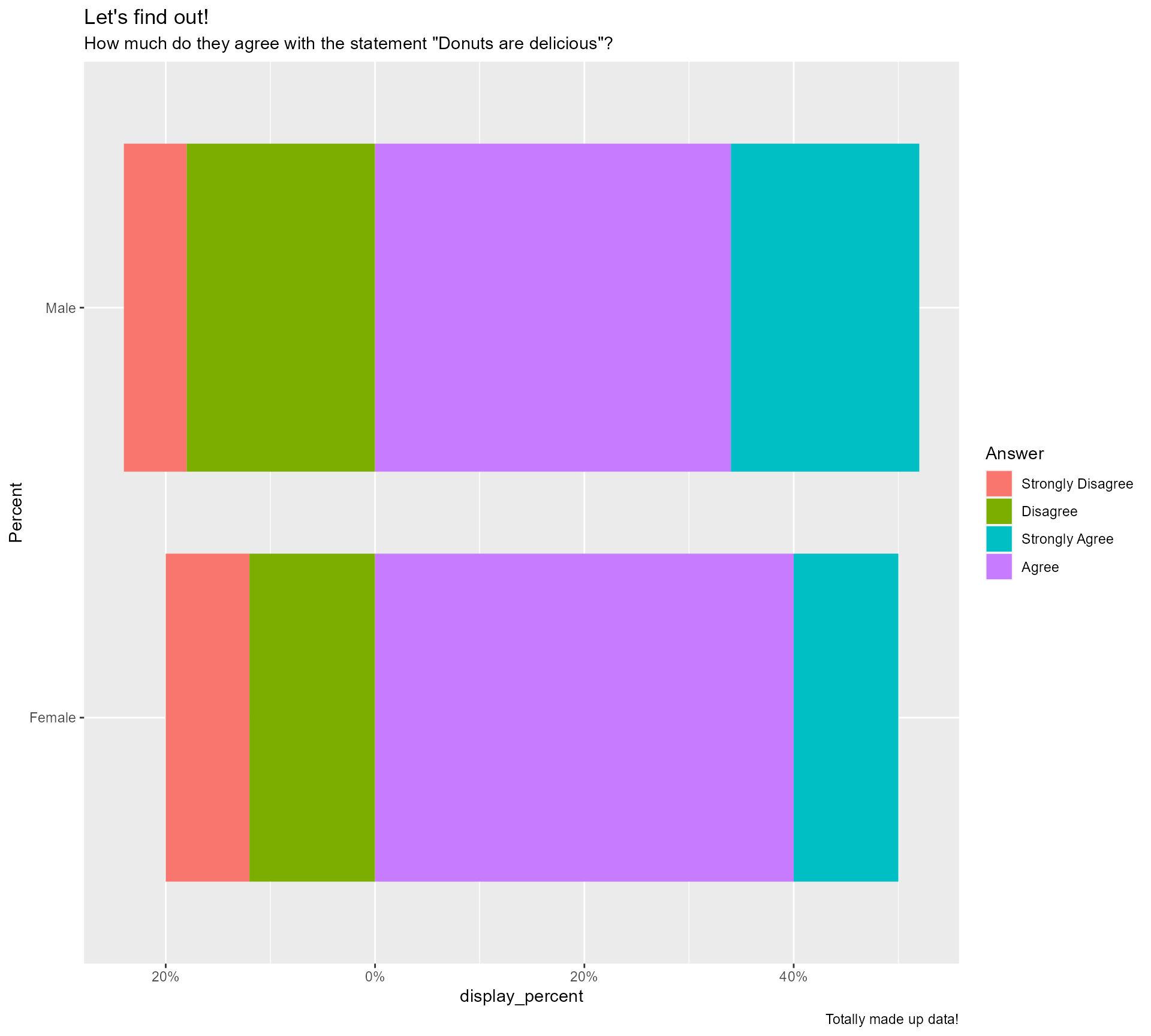
Two extra lines
tibble(answer = factor(rep(c("Strongly Disagree", "Disagree",
                             "Agree", "Strongly Agree"), 2),
                       levels = c("Strongly Disagree", "Disagree",
                                  "Strongly Agree", "Agree")),
       percent = c(8, 12, 40, 10,
                   6, 18, 34, 18),
       group = sort(rep(c("Male", "Female"), 4))) %>%
  mutate(display_percent = case_when(grepl("Dis|Neutral", answer) ~ -percent,
                                     TRUE ~ percent)) %>%
  ggplot() +
  geom_col(aes(x = group,
               fill = answer,
               y = display_percent),
           width = 0.8) +
  labs(title = "Let's find out!",
       subtitle = "How much do they agree with the statement \"Donuts are delicious\"?",
       caption = "Totally made up data!",
       x = "Percent",
       fill = "Answer") +
  scale_y_continuous(labels = function(x) paste0(abs(x), "%")) +
  coord_flip() +
  scale_fill_ophelia(
    palette = "neg_to_pos",
    limits = c("Strongly Disagree", "Disagree",
               "Agree", "Strongly Agree")) +
  theme_ophelia(background_colour = FALSE,
                base_text_size = 14) +
  theme(axis.title = element_blank(),
        legend.position = "bottom")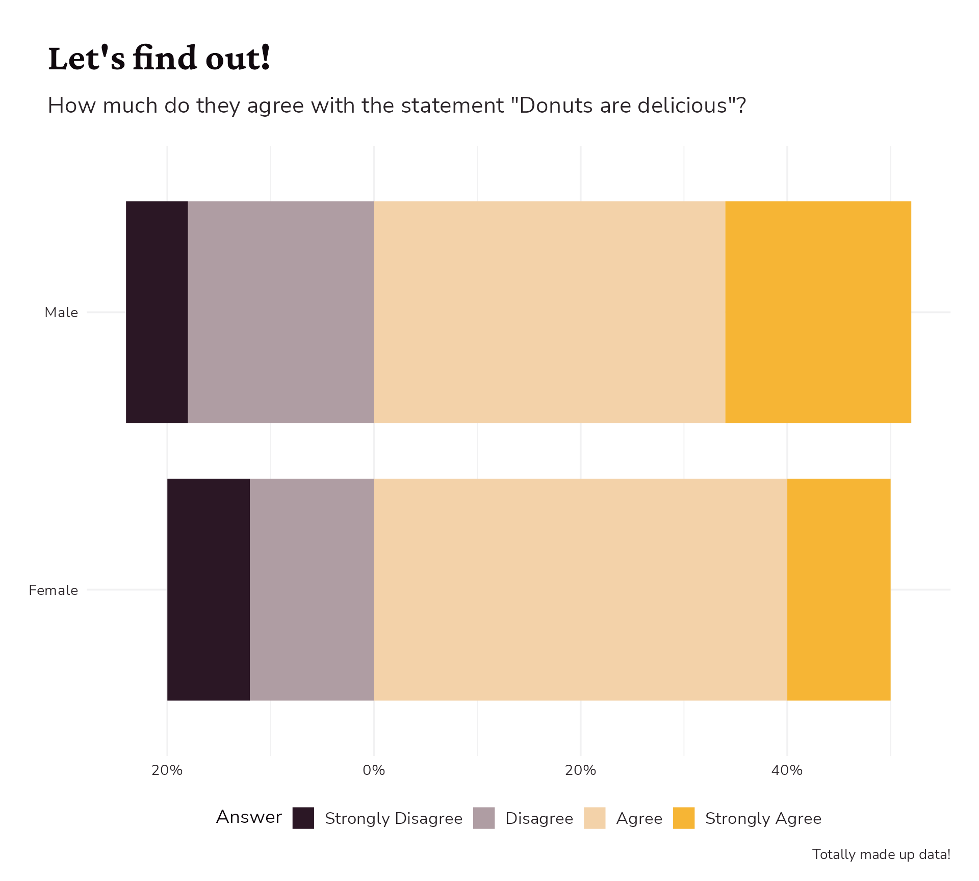
Tada!
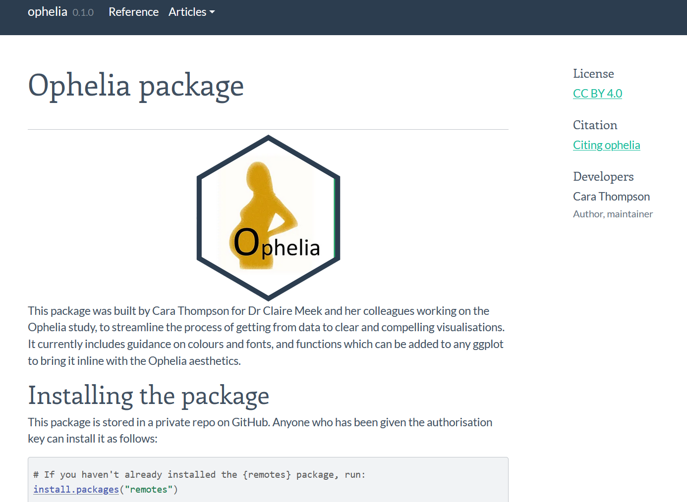
Finalise documentation
Using {pkgdown} - cararthompson.github.io/ophelia/
Keep on building…
Interactive graphs with ggiraph tooltip formatting defaults
palmerpenguins::penguins %>%
  ggplot() +
  geom_point(aes(x = bill_length_mm,
                 y = flipper_length_mm,
                 fill = body_mass_g,
                 size = body_mass_g),
             shape = 21,
             colour = "white",
             alpha = 0.8) +
  labs(x = "Bill length (mm)",
       y = "Flipper length (mm)",
       title = "Perfectly proportional penguins",
       caption = "Data from {palmerpenguins}") +
  guides(size = "none") +
  ophelia::scale_fill_ophelia(continuous = TRUE) +
  ophelia::theme_ophelia()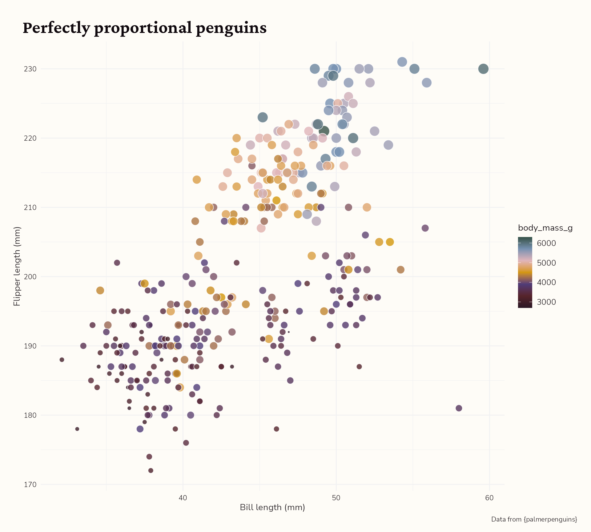
Building Dataviz Design Systems
- Colour scheme
- Set of fonts
ggplottheme- Interactive tables
- Interactive plots
- Quarto slides
- Word/ppt-friendly tables
- Commonly used plots
- …
Over to you!
hello@cararthompson.com
—
Data-to-viz Commissions
Dataviz Design Systems
Training & Consultations
![]()