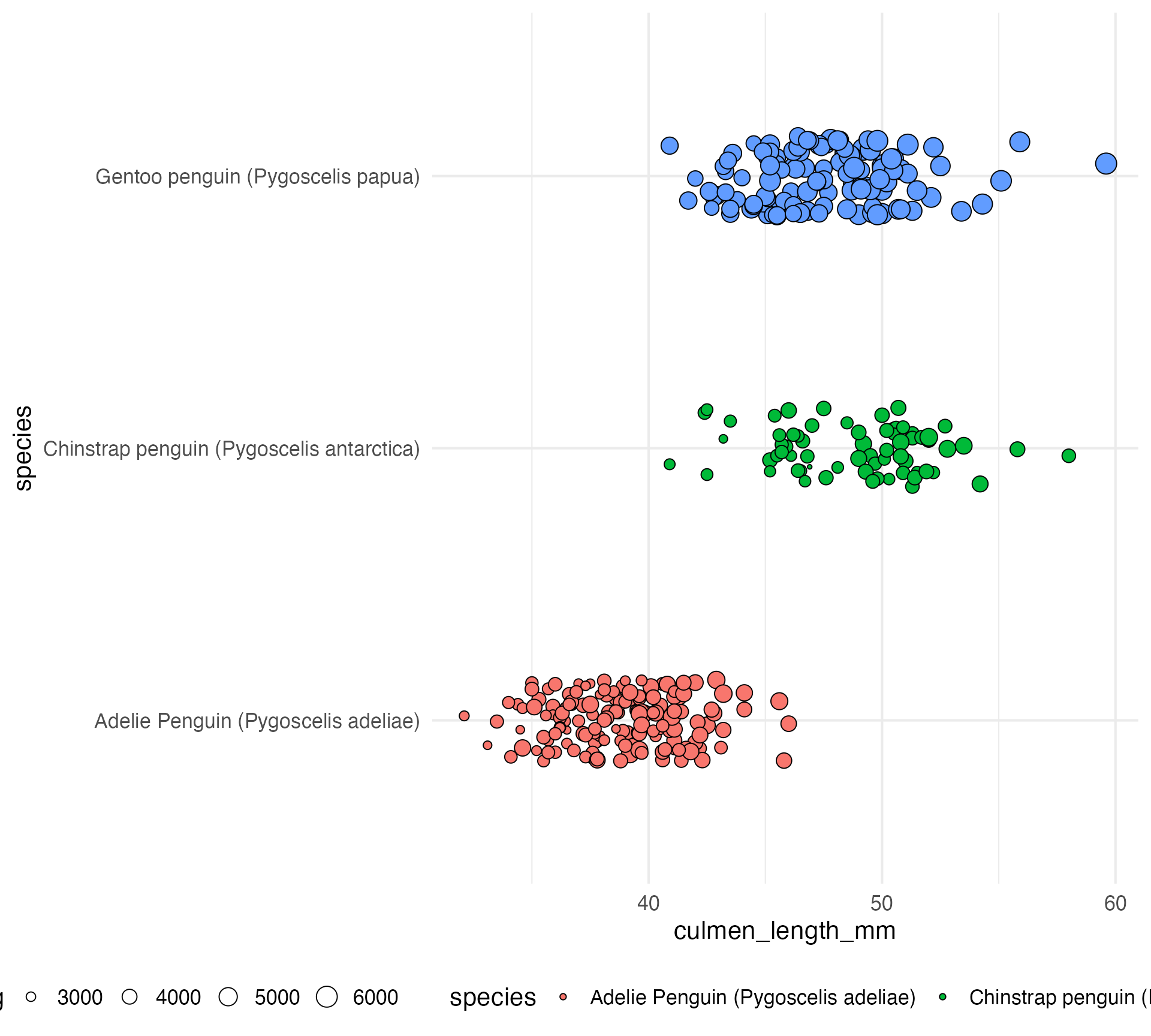
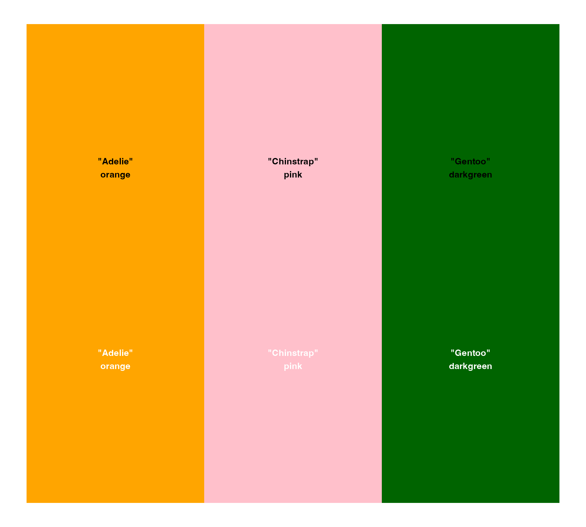
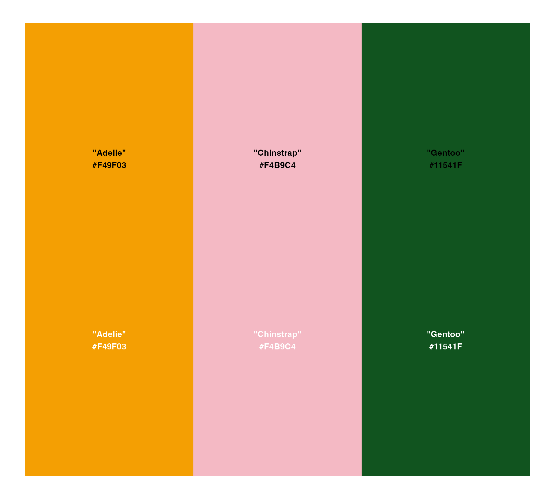
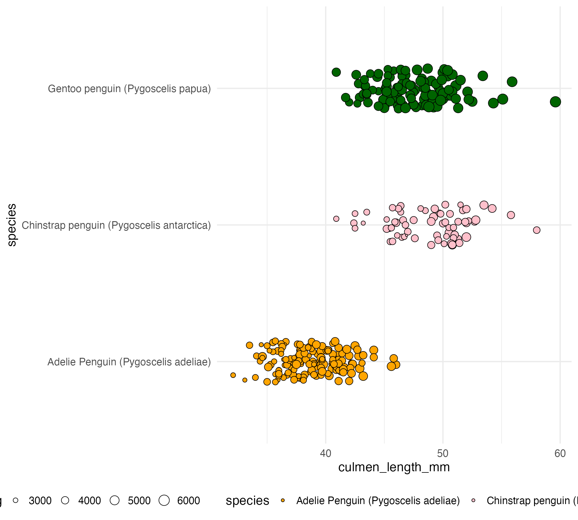
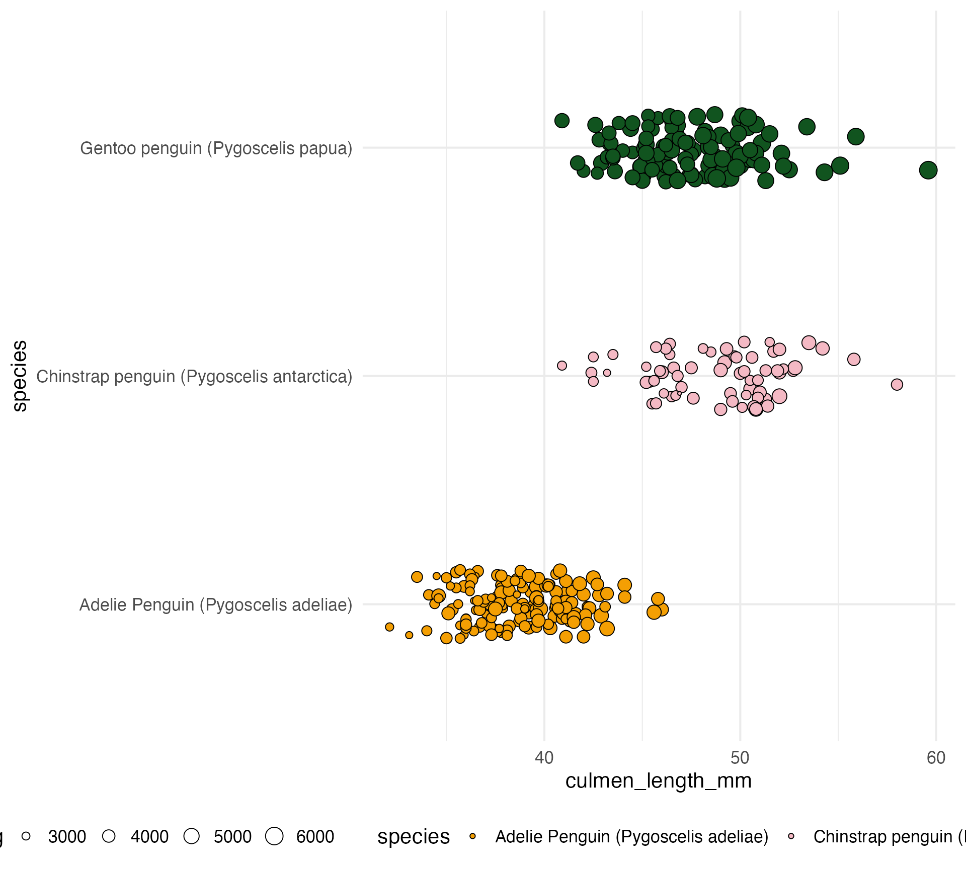
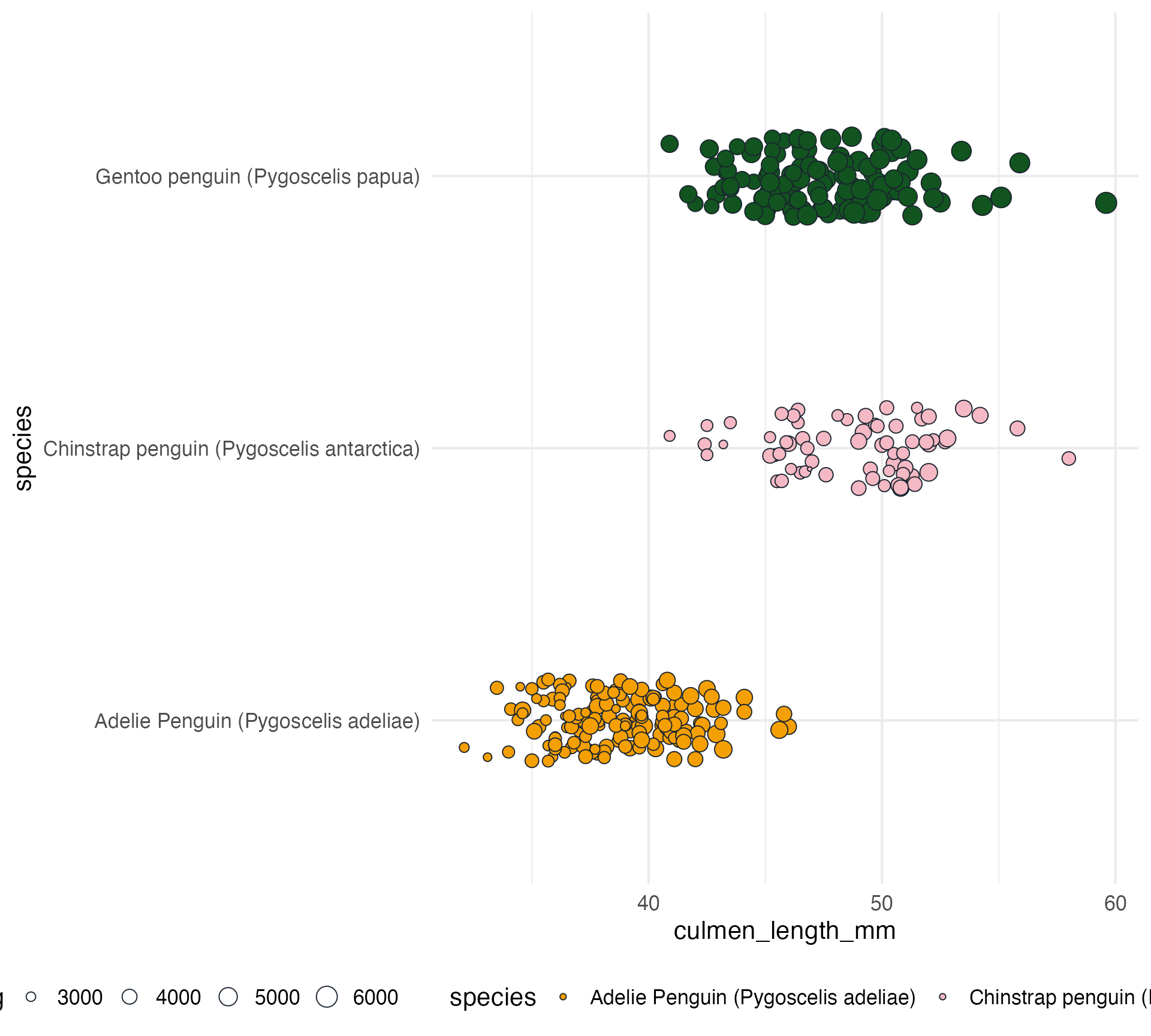
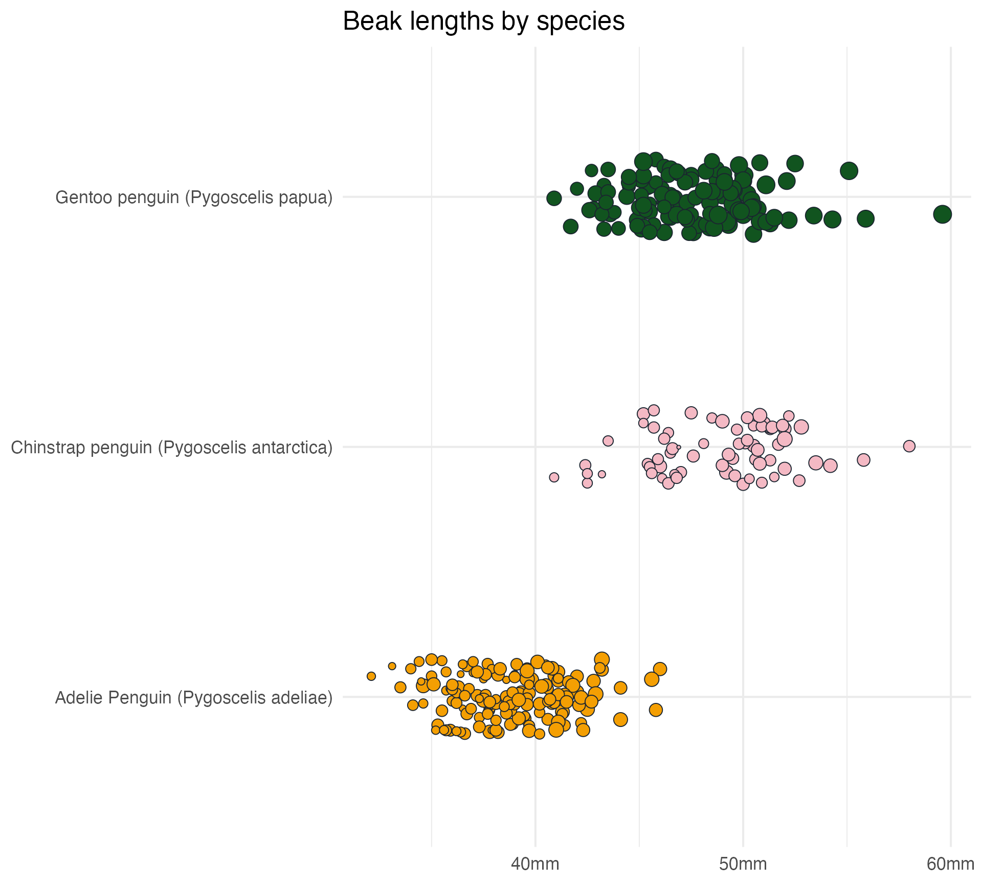
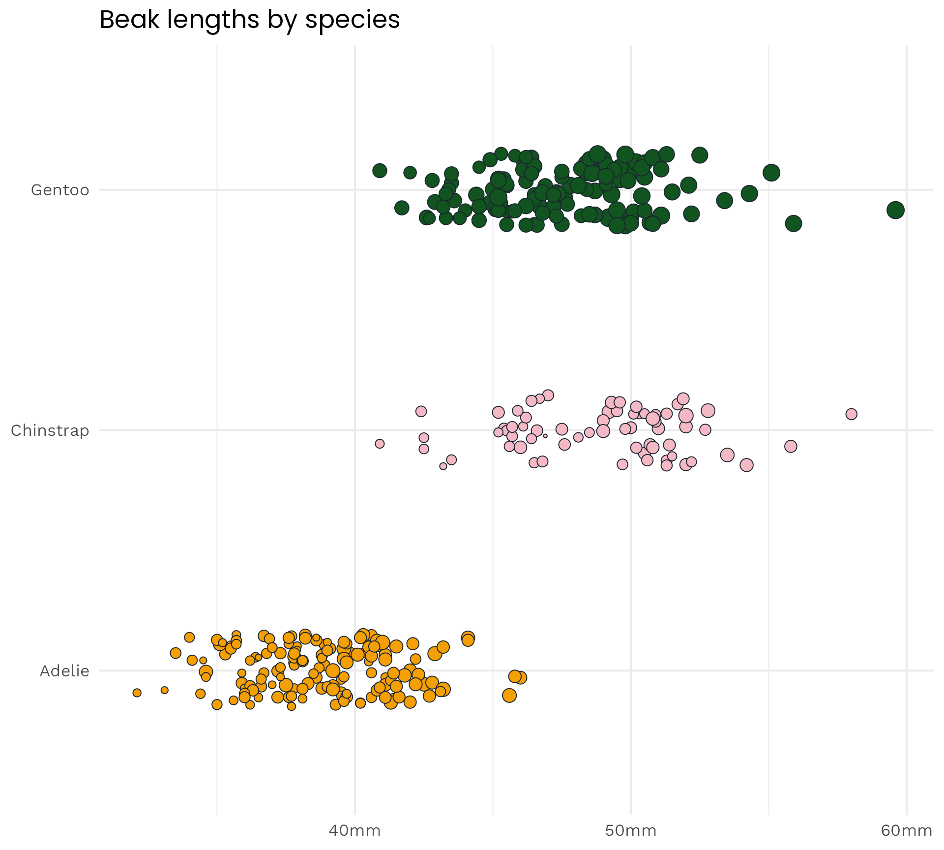
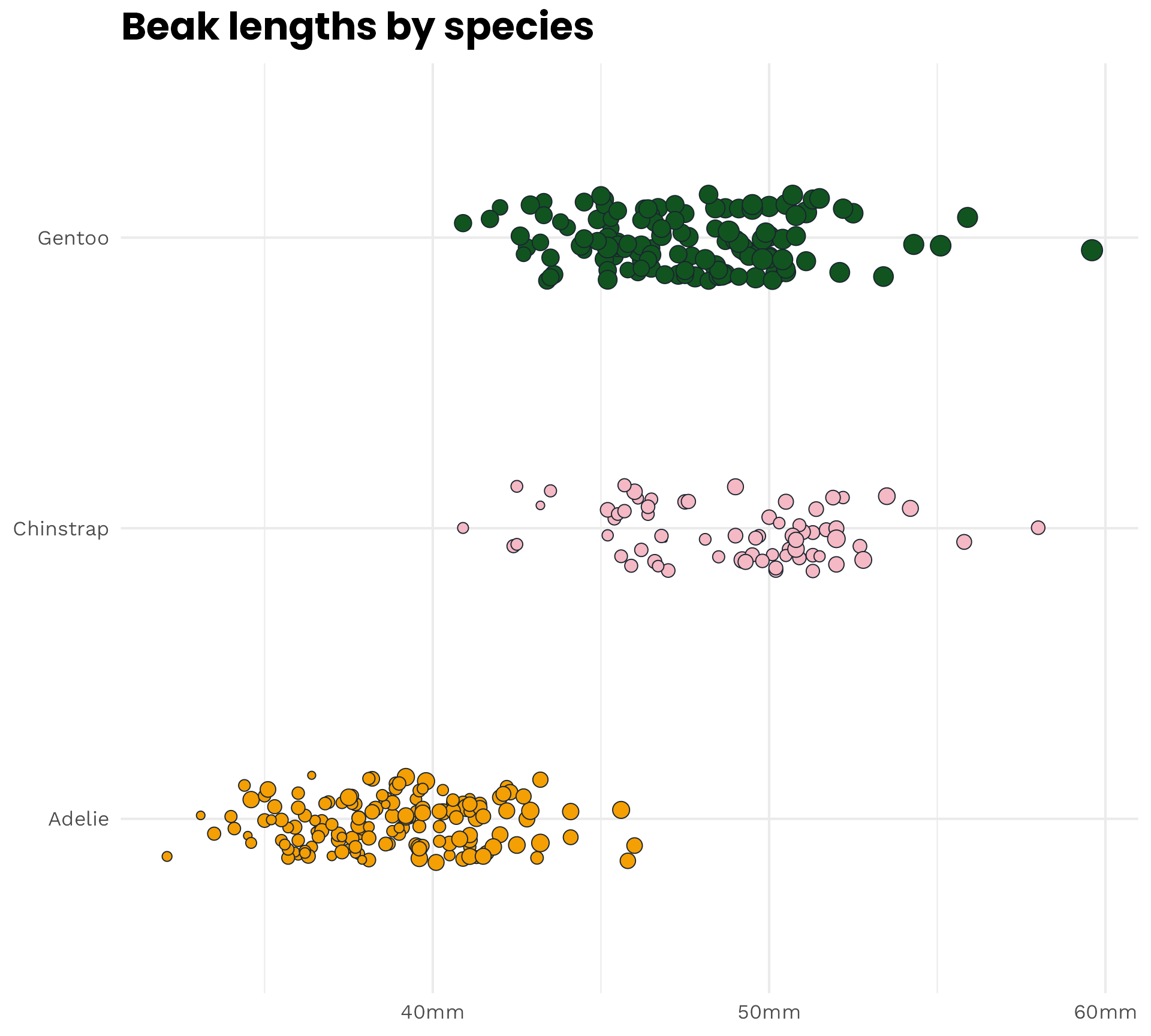
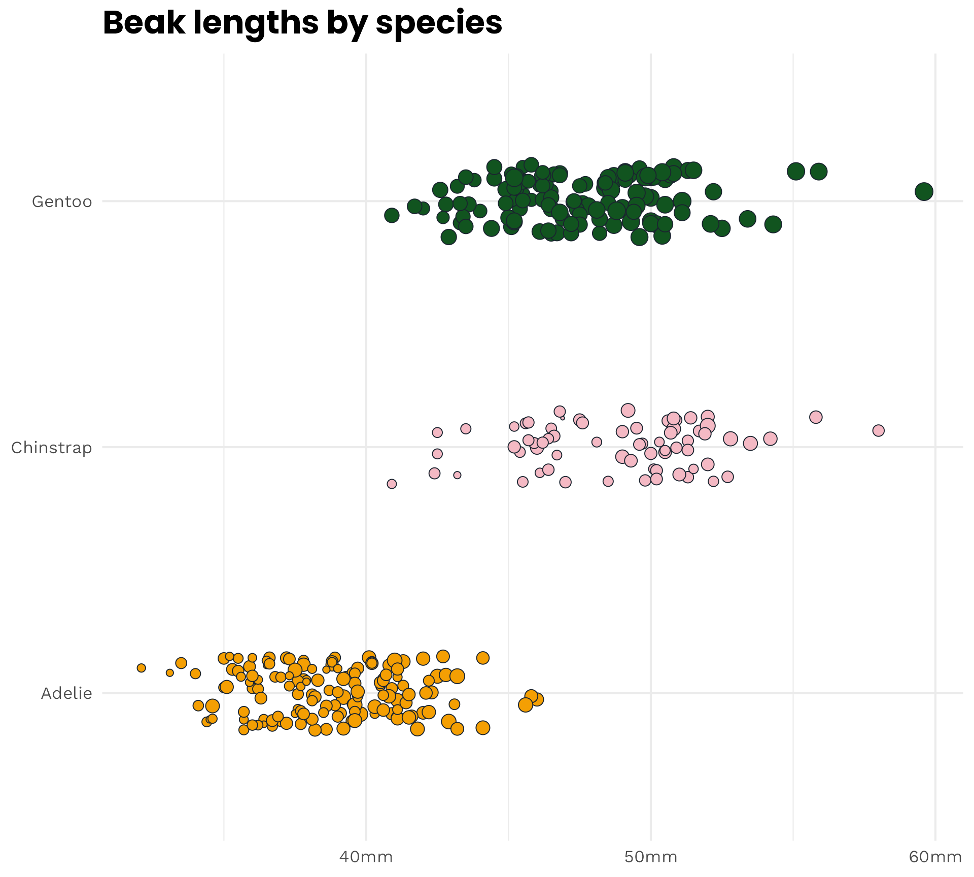
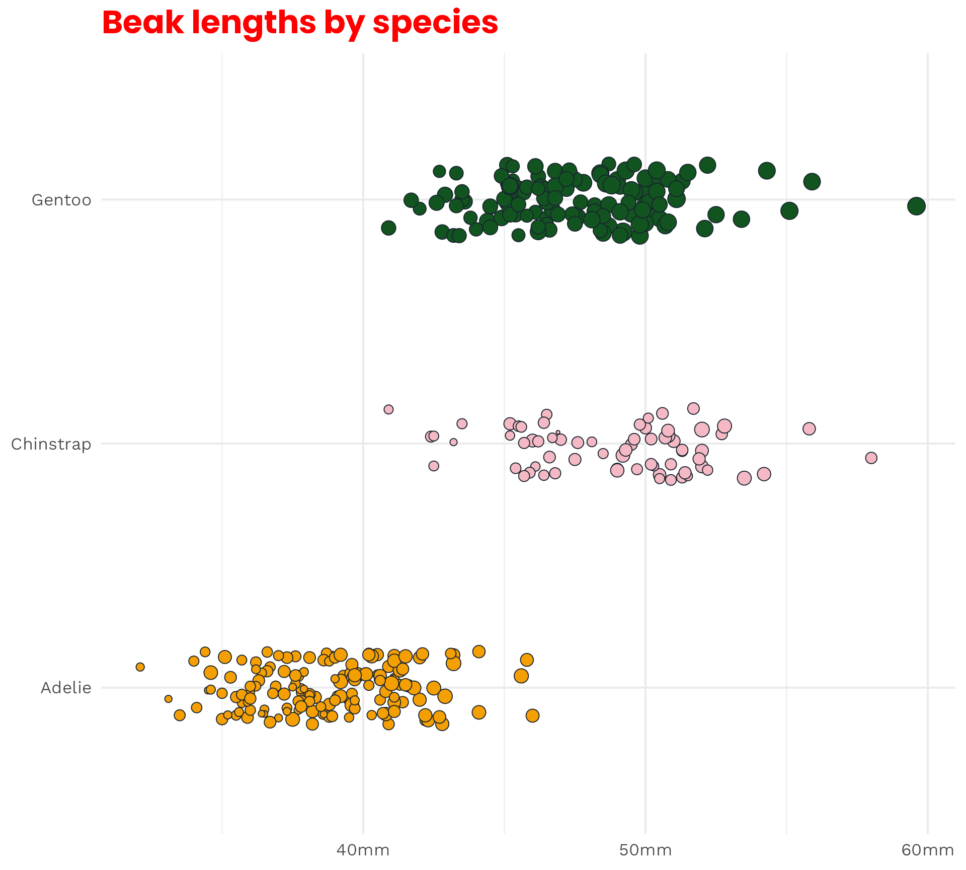
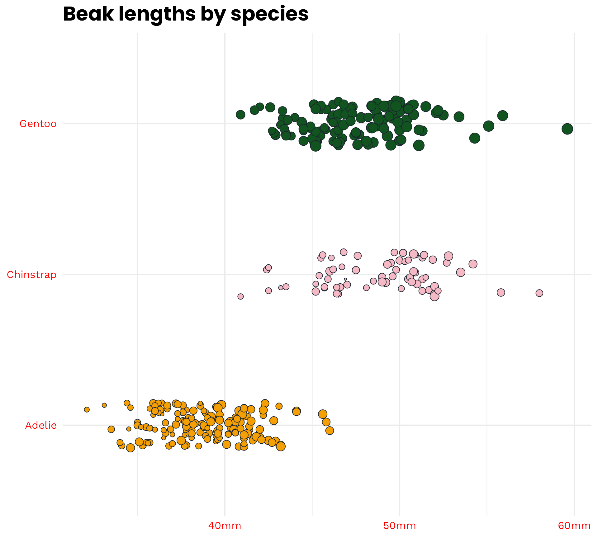
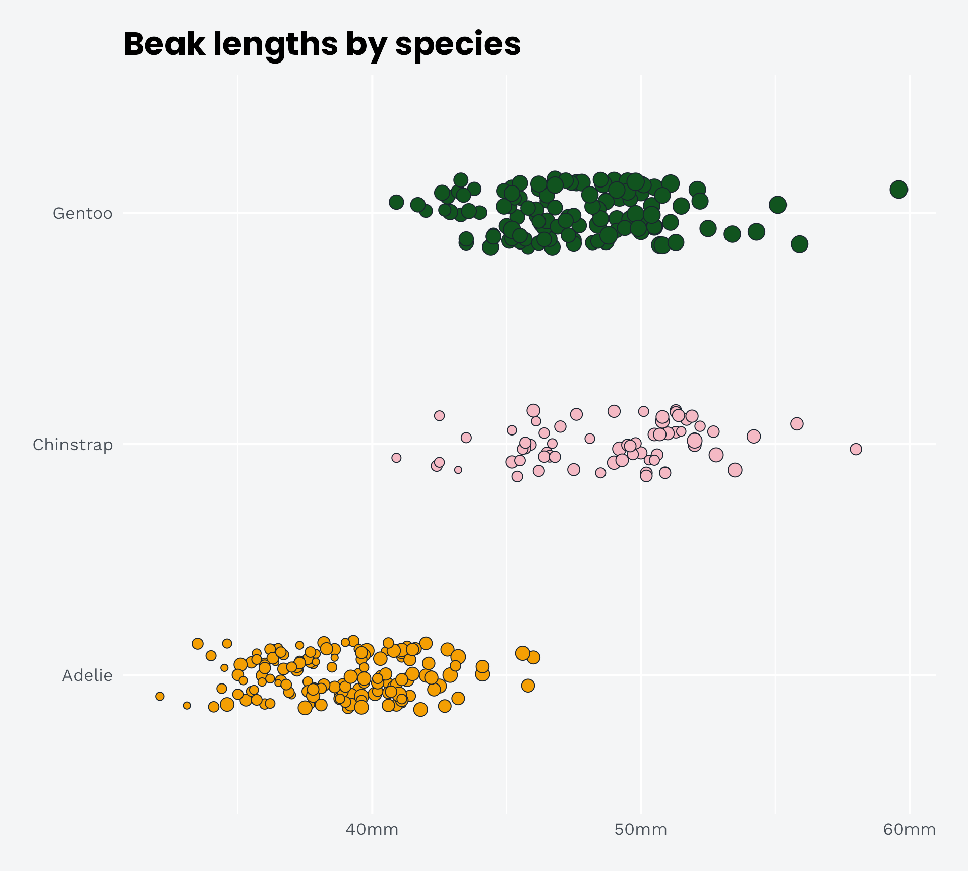
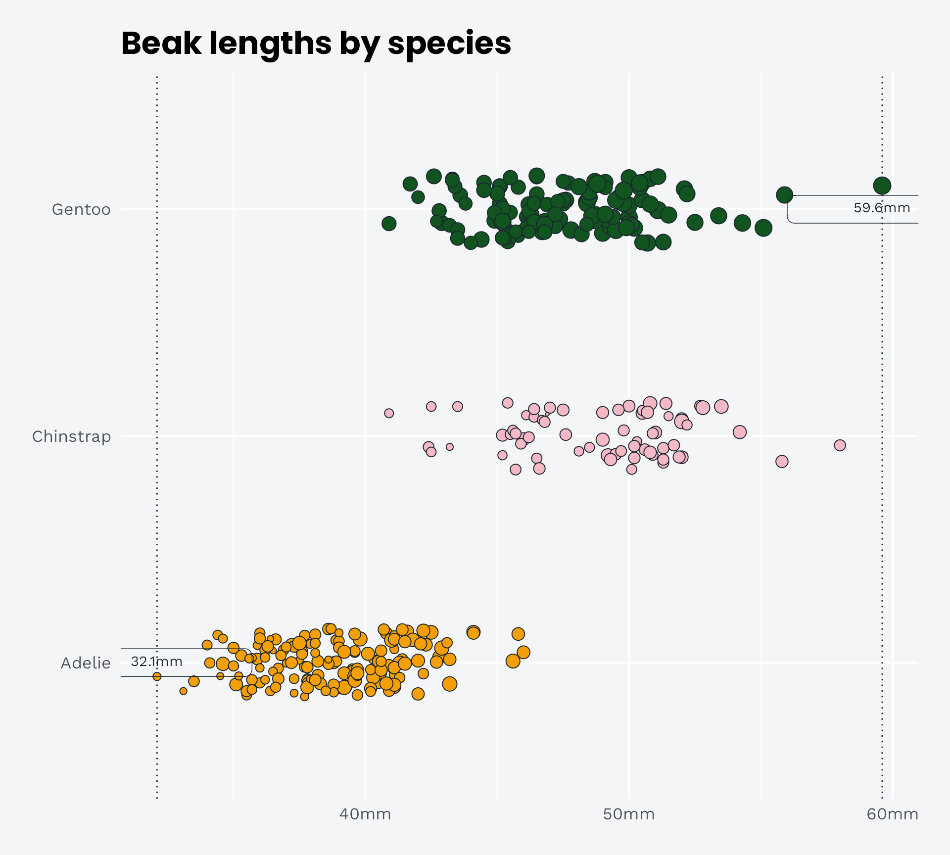
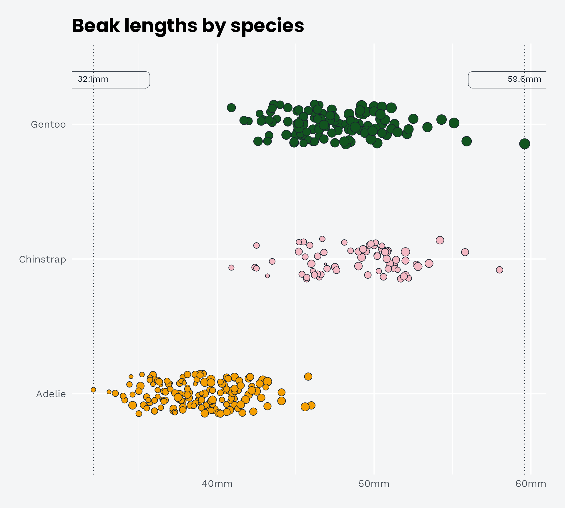
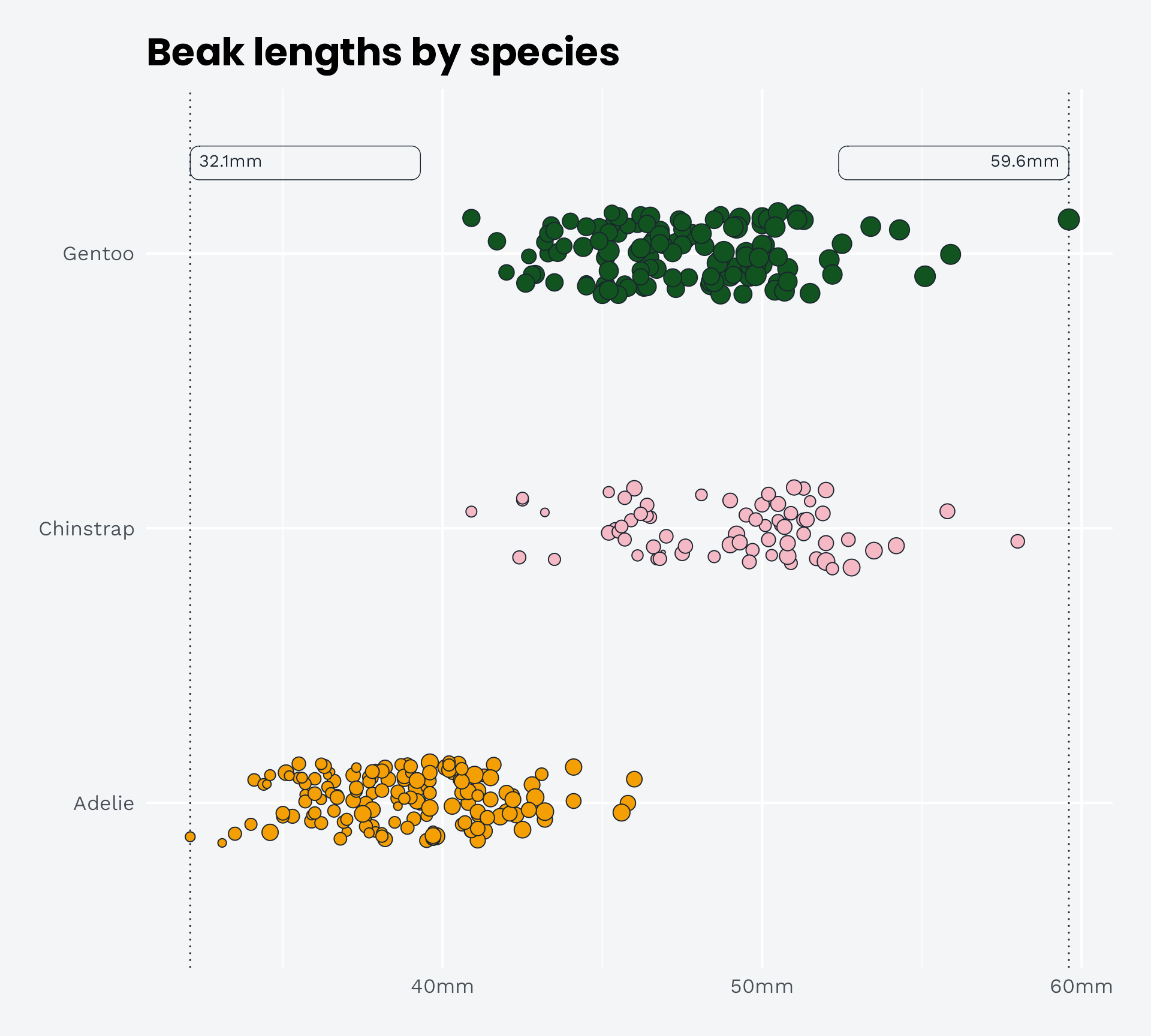
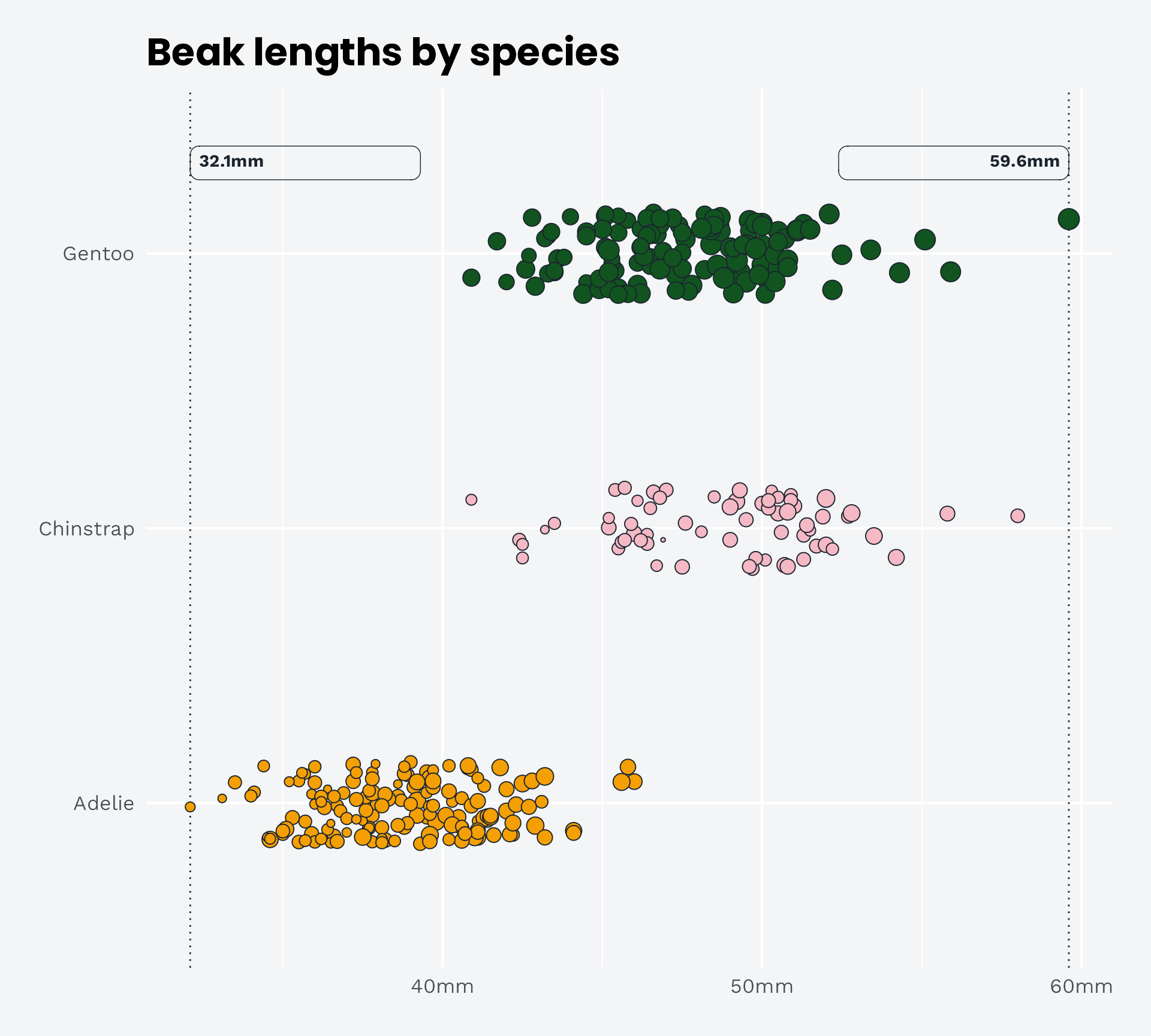
Visualise, Optimise, Parameterise!

The Great Penguin Beak-Off

Cara R Thompson, PhD
RMedicine | 10th June 2025

Hello 👋

👩 Cara Thompson

👩‍💻 Love for patterns in music & language, and a fascination with the human brain %>%

       Psychology PhD %>%

       Analysis of postgraduate medical examinations %>%

       Data Visualisation Consultant

💙 Helping others maximise the impact of their expertise

I ❤️ parameterising dataviz

I ❤️ parameterising dataviz

Why parameterise your plots?

• Reporting on different iterations
• Setting up visualisations before we have all the data
• Comparing different groups/scenarios in your data
• Making life easier for those “can you just?” moments

Why parameterise your plots?

Why parameterise your plots?

What are the traps?

• Colours jumping around
• Axis limits decisions
• Annotations in the wrong place
• Not being able to get hold of a variable we need
• …

Parameterised for…

• Different datasets
• Different presentation contexts
• Different questions
• Clever ID/dataviz matching
• …
• Sanity and code maintenance

The Great Penguin

Beak-Off

Housekeeping

• Code along!
• Using the 📦 {palmerpenguins} penguins
• Using namespacing :: for clarity (and good practice!)
• No silly questions
• Interruptions are welcome
• Slides (incl. code) on my website, code gists shared in the chat

Housekeeping

• Build a plot
• Optimise it with colours, styling & programmatic annotations
• Turn it into a function

Take a break

• Get the penguins into teams and see what we need to tweak
• Explore different parameterisation scenarios

Visualise

What’s the best way to visualise the story?

• Range of beak (culmen) lengths
• Size of teams
• Good representation of the penguin population
• Representative mean within each group

What’s the best way to visualise the story?

• Range of beak (culmen) lengths
• Ideally all three species represented
• Representative mean within each species

Our starting point

Penguin beak lengths by species

library(ggplot2)

palmerpenguins::penguins_raw |>
  janitor::clean_names() |>
  dplyr::filter(!is.na(culmen_length_mm)) |>
  head()

# A tibble: 6 × 17
  study_name sample_number species             region island stage individual_id
  <chr>              <dbl> <chr>               <chr>  <chr>  <chr> <chr>        
1 PAL0708                1 Adelie Penguin (Py… Anvers Torge… Adul… N1A1         
2 PAL0708                2 Adelie Penguin (Py… Anvers Torge… Adul… N1A2         
3 PAL0708                3 Adelie Penguin (Py… Anvers Torge… Adul… N2A1         
4 PAL0708                5 Adelie Penguin (Py… Anvers Torge… Adul… N3A1         
5 PAL0708                6 Adelie Penguin (Py… Anvers Torge… Adul… N3A2         
6 PAL0708                7 Adelie Penguin (Py… Anvers Torge… Adul… N4A1         
# ℹ 10 more variables: clutch_completion <chr>, date_egg <date>,
#   culmen_length_mm <dbl>, culmen_depth_mm <dbl>, flipper_length_mm <dbl>,
#   body_mass_g <dbl>, sex <chr>, delta_15_n_o_oo <dbl>, delta_13_c_o_oo <dbl>,
#   comments <chr>

penguin_df <- palmerpenguins::penguins_raw |>
  janitor::clean_names() |>
  dplyr::filter(!is.na(culmen_length_mm))

Our starting point

Let’s make a graph!

penguin_df |>
  ggplot() +
  geom_point(aes(
    x = culmen_length_mm,
    y = species
  ))

Our starting point

Avoid all the overlaps

penguin_df |>
  ggplot() +
  geom_jitter(
    aes(
      x = culmen_length_mm,
      y = species
    )
  )

Our starting point

Make the grouping clear, and only jitter what doesn’t matter!

penguin_df |>
  ggplot() +
  geom_jitter(
    aes(
      x = culmen_length_mm,
      y = species
    ),
    width = 0,
    height = 0.15
  )

Our starting point

Add a few layers of meaning…

penguin_df |>
  ggplot() +
  geom_jitter(
    aes(
      x = culmen_length_mm,
      y = species,
      fill = species
    ),
    shape = 21,
    width = 0,
    height = 0.15
  )

Our starting point

Add a few layers of meaning…

penguin_df |>
  ggplot() +
  geom_jitter(
    aes(
      x = culmen_length_mm,
      y = species,
      fill = species,
      size = body_mass_g
    ),
    shape = 21,
    width = 0,
    height = 0.15
  )

Our starting point

Too much…?

penguin_df |>
  ggplot() +
  geom_jitter(
    aes(
      x = culmen_length_mm,
      y = species,
      fill = species,
      size = body_mass_g
    ),
    shape = 25,
    width = 0,
    height = 0.15
  )

Our starting point

theme_minimal()

penguin_df |>
  ggplot() +
  geom_jitter(
    aes(
      x = culmen_length_mm,
      y = species,
      fill = species,
      size = body_mass_g
    ),
    shape = 21,
    width = 0,
    height = 0.15
  ) +
  theme_minimal()

Our starting point

theme_minimal()

penguin_df |>
  ggplot() +
  geom_jitter(
    aes(
      x = culmen_length_mm,
      y = species,
      fill = species,
      size = body_mass_g
    ),
    shape = 21,
    width = 0,
    height = 0.15
  ) +
  theme_minimal(base_size = 16)

Our starting point

Move the legend

penguin_df |>
  ggplot() +
  geom_jitter(
    aes(
      x = culmen_length_mm,
      y = species,
      fill = species,
      size = body_mass_g
    ),
    shape = 21,
    width = 0,
    height = 0.15
  ) +
  theme_minimal(base_size = 16) +
  theme(legend.position = "bottom")

Your own code…

• If you have a plot already, great!
• If you don’t, use mine!
• Feel free to pretend it’s about a different topic

Optimise!

Colours, text, annotations (the quick version)

Better colours

Starting with the same letter(ish)

What would your colours be?

Better colours

Blending in a common colour

Better colours

Blending in a common colour - {monochromeR}

Better colours

Blending in a common colour - {monochromeR}

Better colours

It’s subtle… Wait for it!

penguin_df |>
  ggplot() +
  geom_jitter(
    aes(
      x = culmen_length_mm,
      y = species,
      fill = species,
      size = body_mass_g
    ),
    shape = 21,
    width = 0,
    height = 0.15
  ) +
  scale_fill_manual(values = c("orange", "pink", "darkgreen")) +
  theme_minimal(base_size = 16) +
  theme(legend.position = "bottom")

Better colours

It’s subtle… Wait for it!

penguin_df |>
  ggplot() +
  geom_jitter(
    aes(
      x = culmen_length_mm,
      y = species,
      fill = species,
      size = body_mass_g
    ),
    shape = 21,
    width = 0,
    height = 0.15
  ) +
  scale_fill_manual(values = c("#F49F03", "#F4B9C4", "#11541F")) +
  theme_minimal(base_size = 16) +
  theme(legend.position = "bottom")

Better colours

It’s subtle… One last thing for now

penguin_df |>
  ggplot() +
  geom_jitter(
    aes(
      x = culmen_length_mm,
      y = species,
      fill = species,
      size = body_mass_g
    ),
    shape = 21,
    width = 0,
    height = 0.15,
    colour = "#1A242F",
    stroke = 0.5
  ) +
  scale_fill_manual(values = c("#F49F03", "#F4B9C4", "#11541F")) +
  theme_minimal(base_size = 16) +
  theme(legend.position = "bottom")

How come your jitter graphs look different to mine?

Control perception of what belongs together

Better colours

• What are your semantic colours?
• What colour do you need/want to blend in?
• Give it a go!
• monochromeR app

Better text

Do we need the legend? (maybe later?)

penguin_df |>
  ggplot() +
  geom_jitter(
    aes(
      x = culmen_length_mm,
      y = species,
      fill = species,
      size = body_mass_g
    ),
    shape = 21,
    width = 0,
    height = 0.15,
    colour = "#1A242F",
    stroke = 0.5
  ) +
  scale_fill_manual(values = c("#F49F03", "#F4B9C4", "#11541F")) +
  theme_minimal(base_size = 16) +
  theme(legend.position = "none")

Better text

Or the axis titles?

penguin_df |>
  ggplot() +
  geom_jitter(
    aes(
      x = culmen_length_mm,
      y = species,
      fill = species,
      size = body_mass_g
    ),
    shape = 21,
    width = 0,
    height = 0.15,
    colour = "#1A242F",
    stroke = 0.5
  ) +
  scale_fill_manual(values = c("#F49F03", "#F4B9C4", "#11541F")) +
  theme_minimal(base_size = 16) +
  theme(legend.position = "none", axis.title = element_blank())

Better text

What about a title?

penguin_df |>
  ggplot() +
  geom_jitter(
    aes(
      x = culmen_length_mm,
      y = species,
      fill = species,
      size = body_mass_g
    ),
    shape = 21,
    width = 0,
    height = 0.15,
    colour = "#1A242F",
    stroke = 0.5
  ) +
  labs(title = "Beak lengths by species") +
  scale_fill_manual(values = c("#F49F03", "#F4B9C4", "#11541F")) +
  theme_minimal(base_size = 16) +
  theme(legend.position = "none", axis.title = element_blank())

Better text

Let’s be helpful

penguin_df |>
  ggplot() +
  geom_jitter(
    aes(
      x = culmen_length_mm,
      y = species,
      fill = species,
      size = body_mass_g
    ),
    shape = 21,
    width = 0,
    height = 0.15,
    colour = "#1A242F",
    stroke = 0.5
  ) +
  labs(title = "Beak lengths by species") +
  scale_fill_manual(values = c("#F49F03", "#F4B9C4", "#11541F")) +
  scale_x_continuous(label = function(x) paste0(x, "mm")) +
  theme_minimal(base_size = 16) +
  theme(legend.position = "none", axis.title = element_blank())

Better text

Sort out the y axis text - method #1

penguin_df |>
  ggplot() +
  geom_jitter(
    aes(
      x = culmen_length_mm,
      y = species,
      fill = species,
      size = body_mass_g
    ),
    shape = 21,
    width = 0,
    height = 0.15,
    colour = "#1A242F",
    stroke = 0.5
  ) +
  labs(title = "Beak lengths by species") +
  scale_fill_manual(values = c("#F49F03", "#F4B9C4", "#11541F")) +
  scale_x_continuous(label = function(x) paste0(x, "mm")) +
  scale_y_discrete(labels = function(x) gsub("(.)( )(.*)", "\\1", x)) +
  theme_minimal(base_size = 16) +
  theme(legend.position = "none", axis.title = element_blank())

Better text

Sort out the y axis text - method #2

penguin_df |>
  dplyr::mutate(species = gsub("(.)( )(.*)", "\\1", species)) |>
  ggplot() +
  geom_jitter(
    aes(
      x = culmen_length_mm,
      y = species,
      fill = species,
      size = body_mass_g
    ),
    shape = 21,
    width = 0,
    height = 0.15,
    colour = "#1A242F",
    stroke = 0.5
  ) +
  labs(title = "Beak lengths by species") +
  scale_fill_manual(values = c("#F49F03", "#F4B9C4", "#11541F")) +
  scale_x_continuous(label = function(x) paste0(x, "mm")) +
  scale_y_discrete(labels = function(x) gsub("(.)( )(.*)", "\\1", x)) +
  theme_minimal(base_size = 16) +
  theme(legend.position = "none", axis.title = element_blank())

Better text

Better text

Personality

penguin_df |>
  dplyr::mutate(species = gsub("(.)( )(.*)", "\\1", species)) |>
  ggplot() +
  geom_jitter(
    aes(
      x = culmen_length_mm,
      y = species,
      fill = species,
      size = body_mass_g
    ),
    shape = 21,
    width = 0,
    height = 0.15,
    colour = "#1A242F",
    stroke = 0.5
  ) +
  labs(title = "Beak lengths by species") +
  scale_fill_manual(values = c("#F49F03", "#F4B9C4", "#11541F")) +
  scale_x_continuous(label = function(x) paste0(x, "mm")) +
  scale_y_discrete(labels = function(x) gsub("(.)( )(.*)", "\\1", x)) +
  theme_minimal(base_size = 16) +
  theme(
    text = element_text(family = "Work Sans"),
    legend.position = "none",
    axis.title = element_blank(),
    plot.title = element_text(family = "Poppins")
  )

Better text

Personality + hierarchy

penguin_df |>
  dplyr::mutate(species = gsub("(.)( )(.*)", "\\1", species)) |>
  ggplot() +
  geom_jitter(
    aes(
      x = culmen_length_mm,
      y = species,
      fill = species,
      size = body_mass_g
    ),
    shape = 21,
    width = 0,
    height = 0.15,
    colour = "#1A242F",
    stroke = 0.5
  ) +
  labs(title = "Beak lengths by species") +
  scale_fill_manual(values = c("#F49F03", "#F4B9C4", "#11541F")) +
  scale_x_continuous(label = function(x) paste0(x, "mm")) +
  scale_y_discrete(labels = function(x) gsub("(.)( )(.*)", "\\1", x)) +
  theme_minimal(base_size = 16) +
  theme(
    text = element_text(family = "Work Sans"),
    legend.position = "none",
    axis.title = element_blank(),
    plot.title = element_text(
      family = "Poppins", 
      face = "bold", 
      size = 24
    )
  )

Better text

Personality + hierarchy (better!)

penguin_df |>
  dplyr::mutate(species = gsub("(.)( )(.*)", "\\1", species)) |>
  ggplot() +
  geom_jitter(
    aes(
      x = culmen_length_mm,
      y = species,
      fill = species,
      size = body_mass_g
    ),
    shape = 21,
    width = 0,
    height = 0.15,
    colour = "#1A242F",
    stroke = 0.5
  ) +
  labs(title = "Beak lengths by species") +
  scale_fill_manual(values = c("#F49F03", "#F4B9C4", "#11541F")) +
  scale_x_continuous(label = function(x) paste0(x, "mm")) +
  scale_y_discrete(labels = function(x) gsub("(.)( )(.*)", "\\1", x)) +
  theme_minimal(base_size = 16) +
  theme(
    text = element_text(family = "Work Sans"),
    legend.position = "none",
    axis.title = element_blank(),
    plot.title = element_text(
      family = "Poppins",
      face = "bold",
      size = rel(1.5)
    )
  )

Better text

Personality + hierarchy + colour

penguin_df |>
  dplyr::mutate(species = gsub("(.)( )(.*)", "\\1", species)) |>
  ggplot() +
  geom_jitter(
    aes(
      x = culmen_length_mm,
      y = species,
      fill = species,
      size = body_mass_g
    ),
    shape = 21,
    width = 0,
    height = 0.15,
    colour = "#1A242F",
    stroke = 0.5
  ) +
  labs(title = "Beak lengths by species") +
  scale_fill_manual(values = c("#F49F03", "#F4B9C4", "#11541F")) +
  scale_x_continuous(label = function(x) paste0(x, "mm")) +
  scale_y_discrete(labels = function(x) gsub("(.)( )(.*)", "\\1", x)) +
  theme_minimal(base_size = 16) +
  theme(
    text = element_text(family = "Work Sans", colour = "red"),
    legend.position = "none",
    axis.title = element_blank(),
    plot.title = element_text(
      family = "Poppins",
      face = "bold",
      size = rel(1.5)
    )
  )

Better text

??? - theme_minimal()!

penguin_df |>
  dplyr::mutate(species = gsub("(.)( )(.*)", "\\1", species)) |>
  ggplot() +
  geom_jitter(
    aes(
      x = culmen_length_mm,
      y = species,
      fill = species,
      size = body_mass_g
    ),
    shape = 21,
    width = 0,
    height = 0.15,
    colour = "#1A242F",
    stroke = 0.5
  ) +
  labs(title = "Beak lengths by species") +
  scale_fill_manual(values = c("#F49F03", "#F4B9C4", "#11541F")) +
  scale_x_continuous(label = function(x) paste0(x, "mm")) +
  scale_y_discrete(labels = function(x) gsub("(.)( )(.*)", "\\1", x)) +
  theme_minimal(base_size = 16) +
  theme(
    text = element_text(family = "Work Sans"),
    axis.text = element_text(colour = "red"),
    legend.position = "none",
    axis.title = element_blank(),
    plot.title = element_text(
      family = "Poppins",
      face = "bold",
      size = rel(1.5)
    )
  )

Better text

Personality + hierarchy + colour

penguin_df |>
  dplyr::mutate(species = gsub("(.)( )(.*)", "\\1", species)) |>
  ggplot() +
  geom_jitter(
    aes(
      x = culmen_length_mm,
      y = species,
      fill = species,
      size = body_mass_g
    ),
    shape = 21,
    width = 0,
    height = 0.15,
    colour = "#1A242F",
    stroke = 0.5
  ) +
  labs(title = "Beak lengths by species") +
  scale_fill_manual(values = c("#F49F03", "#F4B9C4", "#11541F")) +
  scale_x_continuous(label = function(x) paste0(x, "mm")) +
  scale_y_discrete(labels = function(x) gsub("(.)( )(.*)", "\\1", x)) +
  theme_minimal(base_size = 16) +
  theme(
    text = element_text(family = "Work Sans"),
    axis.text = element_text(colour = "#495058"),
    legend.position = "none",
    axis.title = element_blank(),
    plot.title = element_text(
      family = "Poppins",
      face = "bold",
      size = rel(1.5),
      colour = "#1A242F"
    )
  )

Better text

• Here’s the updated code
• install.packages("systemfonts")
• systemfonts::system_fonts() |> View()
• Pick a different font for your plot
• Change the text colours

Optimise the small things

Background, grid, margins…

penguin_df |>
  dplyr::mutate(species = gsub("(.)( )(.*)", "\\1", species)) |>
  ggplot() +
  geom_jitter(
    aes(
      x = culmen_length_mm,
      y = species,
      fill = species,
      size = body_mass_g
    ),
    shape = 21,
    width = 0,
    height = 0.15,
    colour = "#1A242F",
    stroke = 0.5
  ) +
  labs(title = "Beak lengths by species") +
  scale_fill_manual(values = c("#F49F03", "#F4B9C4", "#11541F")) +
  scale_x_continuous(label = function(x) paste0(x, "mm")) +
  scale_y_discrete(labels = function(x) gsub("(.)( )(.*)", "\\1", x)) +
  theme_minimal(base_size = 16) +
  theme(
    text = element_text(family = "Work Sans"),
    axis.text = element_text(colour = "#495058"),
    legend.position = "none",
    axis.title = element_blank(),
    plot.title = element_text(
      family = "Poppins",
      face = "bold",
      size = rel(1.5),
      colour = "#1A242F"
    ),
    panel.grid = element_line(colour = "#FFFFFF"),
    plot.background = element_rect(fill = "#F4F5F6", colour = "#F4F5F6"),
    plot.caption = element_text(size = rel(0.8), margin = margin(8, 0, 0, 0)),
    plot.margin = margin(rep(24, 4))
  )

Helping your future self

We can turn all that styling into a theme function!

plot +
  theme_minimal(base_size = 16) +
  theme(
    text = element_text(family = "Work Sans"),
    axis.text = element_text(colour = "#495058"),
    legend.position = "none",
    axis.title = element_blank(),
    plot.title = element_text(
      family = "Poppins",
      face = "bold",
      size = rel(1.5)
    ),
    panel.grid = element_line(colour = "#FFFFFF"),
    plot.background = element_rect(fill = "#F4F5F6", colour = "#F4F5F6"),
    plot.caption = element_text(size = rel(0.8), margin = margin(8, 0, 0, 0)),
    plot.margin = margin(rep(24, 4))
  )

Helping your future self

We can turn all that styling into a theme function!

theme_beak_off <- function() {
  theme_minimal(base_size = 16) +
    theme(
      text = element_text(family = "Work Sans"),
      axis.text = element_text(colour = "#495058"),
      legend.position = "none",
      axis.title = element_blank(),
      plot.title = element_text(
        family = "Poppins",
        face = "bold",
        size = rel(1.5)
      ),
      panel.grid = element_line(colour = "#FFFFFF"),
      plot.background = element_rect(fill = "#F4F5F6", colour = "#F4F5F6"),
      plot.caption = element_text(
        size = rel(0.8),
        margin = margin(8, 0, 0, 0)
      ),
      plot.margin = margin(rep(24, 4))
    )
}

Helping your future self

We can turn all that styling into a theme function!

theme_beak_off <- function(base_text_size = 16) {
  theme_minimal(base_size = base_text_size) +
    theme(
      text = element_text(family = "Work Sans"),
      axis.text = element_text(colour = "#495058"),
      legend.position = "none",
      axis.title = element_blank(),
      plot.title = element_text(
        family = "Poppins",
        face = "bold",
        size = rel(1.5)
      ),
      panel.grid = element_line(colour = "#FFFFFF"),
      plot.background = element_rect(fill = "#F4F5F6", colour = "#F4F5F6"),
      plot.caption = element_text(
        size = rel(0.8),
        margin = margin(base_text_size / 2, 0, 0, 0)
      ),
      plot.margin = margin(rep(base_text_size * 1.5, 4))
    )
}

Helping your future self

We can turn all that styling into a theme function!

ggplot(penguin_df) +
  geom_point(aes(x = flipper_length_mm, y = culmen_length_mm)) +
  labs(title = "Perfectly proportional") +
  theme_beak_off()

ggplot(penguin_df) +
  geom_bar(aes(x = island), stat = "count") +
  labs(title = "But the island populations are quite different") +
  theme_beak_off()

Helping your future self

We can turn all that styling into a theme function!

ggplot(penguin_df) +
  geom_point(aes(x = flipper_length_mm, y = culmen_length_mm)) +
  labs(title = "Perfectly proportional") +
  theme_beak_off(base_text_size = 12)

ggplot(penguin_df) +
  geom_bar(aes(x = island), stat = "count") +
  labs(title = "But the island populations\nare quite different") +
  theme_beak_off(base_text_size = 30)

Helping your future self

• Use my theme function as a starting point
• Change a few things
• Apply it to a different graph altogether!

Annotations

• Main story (range)
• Means within each group
• Programmatic title

Annotations

We need to create some different data…

penguin_df |>
  dplyr::mutate(species = gsub("(.)( )(.*)", "\\1", species)) |>
  ggplot() +
  geom_jitter(
    aes(
      x = culmen_length_mm,
      y = species,
      fill = species,
      size = body_mass_g
    ),
    shape = 21,
    width = 0,
    height = 0.15,
    colour = "#1A242F",
    stroke = 0.5
  ) +
  labs(title = "Beak lengths by species") +
  scale_fill_manual(values = c("#F49F03", "#F4B9C4", "#11541F")) +
  scale_x_continuous(label = function(x) paste0(x, "mm")) +
  theme_beak_off()

Annotations

We need to create some different data…

beak_range_df <- penguin_df |>
  dplyr::mutate(species = gsub("(.)( )(.*)", "\\1", species)) |>
  dplyr::filter(
    culmen_length_mm == max(culmen_length_mm, na.rm = TRUE) |
      culmen_length_mm == min(culmen_length_mm, na.rm = TRUE)
  )

penguin_df |>
  dplyr::mutate(species = gsub("(.)( )(.*)", "\\1", species)) |>
  ggplot() +
  geom_jitter(
    aes(
      x = culmen_length_mm,
      y = species,
      fill = species,
      size = body_mass_g
    ),
    shape = 21,
    width = 0,
    height = 0.15,
    colour = "#1A242F",
    stroke = 0.5
  ) +
  geom_vline(
    data = beak_range_df,
    aes(xintercept = culmen_length_mm),
    linetype = 3
  ) +
  labs(title = "Beak lengths by species") +
  scale_fill_manual(values = c("#F49F03", "#F4B9C4", "#11541F")) +
  scale_x_continuous(label = function(x) paste0(x, "mm")) +
  theme_beak_off()

Annotations

Move to background + change colour

penguin_df |>
  dplyr::mutate(species = gsub("(.)( )(.*)", "\\1", species)) |>
  ggplot() +
  geom_vline(
    data = beak_range_df,
    aes(xintercept = culmen_length_mm),
    linetype = 3,
    colour = "#1A242F"
  ) +
  geom_jitter(
    aes(
      x = culmen_length_mm,
      y = species,
      fill = species,
      size = body_mass_g
    ),
    shape = 21,
    width = 0,
    height = 0.15,
    colour = "#1A242F",
    stroke = 0.5
  ) +
  labs(title = "Beak lengths by species") +
  scale_fill_manual(values = c("#F49F03", "#F4B9C4", "#11541F")) +
  scale_x_continuous(label = function(x) paste0(x, "mm")) +
  theme_beak_off()

Annotations

Add labels

penguin_df |>
  dplyr::mutate(species = gsub("(.)( )(.*)", "\\1", species)) |>
  ggplot(aes(x = culmen_length_mm, y = species)) +
  geom_vline(
    data = beak_range_df,
    aes(xintercept = culmen_length_mm),
    linetype = 3,
    colour = "#1A242F"
  ) +
  geom_jitter(
    aes(
      x = culmen_length_mm,
      y = species,
      fill = species,
      size = body_mass_g
    ),
    shape = 21,
    width = 0,
    height = 0.15,
    colour = "#1A242F",
    stroke = 0.5
  ) +
  ggtext::geom_textbox(
    data = beak_range_df,
    aes(label = paste0(culmen_length_mm, "mm"))
  ) +
  labs(title = "Beak lengths by species") +
  scale_fill_manual(values = c("#F49F03", "#F4B9C4", "#11541F")) +
  scale_x_continuous(label = function(x) paste0(x, "mm")) +
  theme_beak_off()

Annotations

Add labels

penguin_df |>
  dplyr::mutate(species = gsub("(.)( )(.*)", "\\1", species)) |>
  ggplot(aes(x = culmen_length_mm, y = species)) +
  geom_vline(
    data = beak_range_df,
    aes(xintercept = culmen_length_mm),
    linetype = 3,
    colour = "#1A242F"
  ) +
  geom_jitter(
    aes(
      x = culmen_length_mm,
      y = species,
      fill = species,
      size = body_mass_g
    ),
    shape = 21,
    width = 0,
    height = 0.15,
    colour = "#1A242F",
    stroke = 0.5
  ) +
  ggtext::geom_textbox(
    data = beak_range_df,
    aes(label = paste0(culmen_length_mm, "mm")),
    family = "Work Sans",
    halign = 0.5,
    colour = "#1A242F",
    fill = NA
  ) +
  labs(title = "Beak lengths by species") +
  scale_fill_manual(values = c("#F49F03", "#F4B9C4", "#11541F")) +
  scale_x_continuous(label = function(x) paste0(x, "mm")) +
  theme_beak_off()

Annotations

Shift them out of the way of the data

penguin_df |>
  dplyr::mutate(species = gsub("(.)( )(.*)", "\\1", species)) |>
  ggplot(aes(x = culmen_length_mm, y = species)) +
  geom_vline(
    data = beak_range_df,
    aes(xintercept = culmen_length_mm),
    linetype = 3,
    colour = "#1A242F"
  ) +
  geom_jitter(
    aes(
      x = culmen_length_mm,
      y = species,
      fill = species,
      size = body_mass_g
    ),
    shape = 21,
    width = 0,
    height = 0.15,
    colour = "#1A242F",
    stroke = 0.5
  ) +
  ggtext::geom_textbox(
    data = beak_range_df,
    aes(y = max(species), label = paste0(culmen_length_mm, "mm")),
    family = "Work Sans",
    halign = 0.5,
    colour = "#1A242F",
    fill = NA,
    nudge_y = 0.33
  ) +
  labs(title = "Beak lengths by species") +
  scale_fill_manual(values = c("#F49F03", "#F4B9C4", "#11541F")) +
  scale_x_continuous(label = function(x) paste0(x, "mm")) +
  theme_beak_off()

Annotations

Align them sensibly

penguin_df |>
  dplyr::mutate(species = gsub("(.)( )(.*)", "\\1", species)) |>
  ggplot(aes(x = culmen_length_mm, y = species)) +
  geom_vline(
    data = beak_range_df,
    aes(xintercept = culmen_length_mm),
    linetype = 3,
    colour = "#1A242F"
  ) +
  geom_jitter(
    aes(
      x = culmen_length_mm,
      y = species,
      fill = species,
      size = body_mass_g
    ),
    shape = 21,
    width = 0,
    height = 0.15,
    colour = "#1A242F",
    stroke = 0.5
  ) +
  ggtext::geom_textbox(
    data = beak_range_df,
    aes(
      y = max(species),
      label = paste0(culmen_length_mm, "mm"),
      hjust = dplyr::case_when(
        culmen_length_mm == min(culmen_length_mm) ~ 0,
        TRUE ~ 1
      ),
      halign = dplyr::case_when(
        culmen_length_mm == min(culmen_length_mm) ~ 0,
        TRUE ~ 1
      )
    ),
    family = "Work Sans",
    colour = "#1A242F",
    fill = NA,
    nudge_y = 0.33
  ) +
  labs(title = "Beak lengths by species") +
  scale_fill_manual(values = c("#F49F03", "#F4B9C4", "#11541F")) +
  scale_x_continuous(label = function(x) paste0(x, "mm")) +
  theme_beak_off()

Annotations

Add labels

penguin_df |>
  dplyr::mutate(species = gsub("(.)( )(.*)", "\\1", species)) |>
  ggplot(aes(x = culmen_length_mm, y = species)) +
  geom_vline(
    data = beak_range_df,
    aes(xintercept = culmen_length_mm),
    linetype = 3,
    colour = "#1A242F"
  ) +
  geom_jitter(
    aes(
      x = culmen_length_mm,
      y = species,
      fill = species,
      size = body_mass_g
    ),
    shape = 21,
    width = 0,
    height = 0.15,
    colour = "#1A242F",
    stroke = 0.5
  ) +
  ggtext::geom_textbox(
    data = beak_range_df,
    aes(
      y = max(species),
      label = paste0(culmen_length_mm, "mm"),
      hjust = dplyr::case_when(
        culmen_length_mm == min(culmen_length_mm) ~ 0,
        TRUE ~ 1
      ),
      halign = dplyr::case_when(
        culmen_length_mm == min(culmen_length_mm) ~ 0,
        TRUE ~ 1
      )
    ),
    family = "Work Sans",
    colour = "#1A242F",
    fontface = "bold",
    fill = NA,
    nudge_y = 0.33
  ) +
  labs(title = "Beak lengths by species") +
  scale_fill_manual(values = c("#F49F03", "#F4B9C4", "#11541F")) +
  scale_x_continuous(label = function(x) paste0(x, "mm")) +
  theme_beak_off()

Annotations

Improve even more!

penguin_df |>
  dplyr::mutate(species = gsub("(.)( )(.*)", "\\1", species)) |>
  ggplot(aes(x = culmen_length_mm, y = species)) +
  geom_vline(
    data = beak_range_df,
    aes(xintercept = culmen_length_mm),
    linetype = 3,
    colour = "#1A242F"
  ) +
  geom_jitter(
    aes(
      x = culmen_length_mm,
      y = species,
      fill = species,
      size = body_mass_g
    ),
    shape = 21,
    width = 0,
    height = 0.15,
    colour = "#1A242F",
    stroke = 0.5
  ) +
  ggtext::geom_textbox(
    data = beak_range_df,
    aes(
      y = max(species),
      label = dplyr::case_when(
        culmen_length_mm == min(culmen_length_mm) ~
          paste0("🞀 ", culmen_length_mm, "mm"),
        TRUE ~ paste0(culmen_length_mm, "mm", " 🞂")
      ),
      hjust = dplyr::case_when(
        culmen_length_mm == min(culmen_length_mm) ~ 0,
        TRUE ~ 1
      ),
      halign = dplyr::case_when(
        culmen_length_mm == min(culmen_length_mm) ~ 0,
        TRUE ~ 1
      )
    ),
    family = "Work Sans",
    colour = "#1A242F",
    fontface = "bold",
    fill = NA,
    nudge_y = 0.33
  ) +
  labs(title = "Beak lengths by species") +
  scale_fill_manual(values = c("#F49F03", "#F4B9C4", "#11541F")) +
  scale_x_continuous(label = function(x) paste0(x, "mm")) +
  theme_beak_off()

Annotations

Improve even more!

penguin_df |>
  dplyr::mutate(species = gsub("(.)( )(.*)", "\\1", species)) |>
  ggplot(aes(x = culmen_length_mm, y = species)) +
  geom_vline(
    data = beak_range_df,
    aes(xintercept = culmen_length_mm),
    linetype = 3,
    colour = "#1A242F"
  ) +
  geom_jitter(
    aes(
      x = culmen_length_mm,
      y = species,
      fill = species,
      size = body_mass_g
    ),
    shape = 21,
    width = 0,
    height = 0.15,
    colour = "#1A242F",
    stroke = 0.5
  ) +
  ggtext::geom_textbox(
    data = beak_range_df,
    aes(
      y = max(species),
      label = dplyr::case_when(
        culmen_length_mm == min(culmen_length_mm) ~
          paste0("🞀 ", culmen_length_mm, "mm"),
        TRUE ~ paste0(culmen_length_mm, "mm", " 🞂")
      ),
      hjust = dplyr::case_when(
        culmen_length_mm == min(culmen_length_mm) ~ 0,
        TRUE ~ 1
      ),
      halign = dplyr::case_when(
        culmen_length_mm == min(culmen_length_mm) ~ 0,
        TRUE ~ 1
      )
    ),
    family = "Work Sans",
    colour = "#1A242F",
    fontface = "bold",
    fill = NA,
    box.padding = unit(0, "pt"),
    box.colour = NA,
    nudge_y = 0.33
  ) +
  labs(title = "Beak lengths by species") +
  scale_fill_manual(values = c("#F49F03", "#F4B9C4", "#11541F")) +
  scale_x_continuous(label = function(x) paste0(x, "mm")) +
  theme_beak_off()

Annotations

And let’s add a bit more data…

beak_means_df <- penguin_df |>
  dplyr::mutate(species = gsub("(.)( )(.*)", "\\1", species)) |>
  dplyr::group_by(species) |>
  dplyr::summarise(mean_length = mean(culmen_length_mm, na.rm = TRUE))

penguin_df |>
  dplyr::mutate(species = gsub("(.)( )(.*)", "\\1", species)) |>
  ggplot(aes(x = culmen_length_mm, y = species)) +
  geom_vline(
    data = beak_range_df,
    aes(xintercept = culmen_length_mm),
    linetype = 3,
    colour = "#1A242F"
  ) +
  geom_segment(
    data = beak_means_df,
    aes(x = mean_length, xend = mean_length, y = -Inf, yend = species),
    linetype = 3
  ) +
  geom_jitter(
    aes(
      x = culmen_length_mm,
      y = species,
      fill = species,
      size = body_mass_g
    ),
    shape = 21,
    width = 0,
    height = 0.15,
    colour = "#1A242F",
    stroke = 0.5
  ) +
  ggtext::geom_textbox(
    data = beak_range_df,
    aes(
      y = max(species),
      label = dplyr::case_when(
        culmen_length_mm == min(culmen_length_mm) ~
          paste0("🞀 ", culmen_length_mm, "mm"),
        TRUE ~ paste0(culmen_length_mm, "mm", " 🞂")
      ),
      hjust = dplyr::case_when(
        culmen_length_mm == min(culmen_length_mm) ~ 0,
        TRUE ~ 1
      ),
      halign = dplyr::case_when(
        culmen_length_mm == min(culmen_length_mm) ~ 0,
        TRUE ~ 1
      )
    ),
    family = "Work Sans",
    colour = "#1A242F",
    fontface = "bold",
    fill = NA,
    box.padding = unit(0, "pt"),
    box.colour = NA,
    nudge_y = 0.33
  ) +
  ggtext::geom_textbox(
    data = beak_means_df,
    aes(
      x = mean_length,
      y = species,
      label = paste0(
        species,
        " mean<br>**",
        janitor::round_half_up(mean_length),
        "mm**"
      )
    ),
    hjust = 0,
    nudge_y = -0.3,
    box.colour = NA,
    family = "Work Sans",
    colour = "#1A242F",
    fill = "#F4F5F6"
  ) +
  labs(title = "Beak lengths by species") +
  scale_fill_manual(values = c("#F49F03", "#F4B9C4", "#11541F")) +
  scale_x_continuous(label = function(x) paste0(x, "mm")) +
  theme_beak_off()

Annotations

And we can get rid of the y axis!

penguin_df |>
  dplyr::mutate(species = gsub("(.)( )(.*)", "\\1", species)) |>
  ggplot(aes(x = culmen_length_mm, y = species)) +
  geom_vline(
    data = beak_range_df,
    aes(xintercept = culmen_length_mm),
    linetype = 3,
    colour = "#1A242F"
  ) +
  geom_segment(
    data = beak_means_df,
    aes(x = mean_length, xend = mean_length, y = -Inf, yend = species),
    linetype = 3
  ) +
  geom_jitter(
    aes(
      x = culmen_length_mm,
      y = species,
      fill = species,
      size = body_mass_g
    ),
    shape = 21,
    width = 0,
    height = 0.15,
    colour = "#1A242F",
    stroke = 0.5
  ) +
  ggtext::geom_textbox(
    data = beak_range_df,
    aes(
      y = max(species),
      label = dplyr::case_when(
        culmen_length_mm == min(culmen_length_mm) ~
          paste0("🞀 ", culmen_length_mm, "mm"),
        TRUE ~ paste0(culmen_length_mm, "mm", " 🞂")
      ),
      hjust = dplyr::case_when(
        culmen_length_mm == min(culmen_length_mm) ~ 0,
        TRUE ~ 1
      ),
      halign = dplyr::case_when(
        culmen_length_mm == min(culmen_length_mm) ~ 0,
        TRUE ~ 1
      )
    ),
    family = "Work Sans",
    colour = "#1A242F",
    fontface = "bold",
    fill = NA,
    box.padding = unit(0, "pt"),
    box.colour = NA,
    nudge_y = 0.33
  ) +
  ggtext::geom_textbox(
    data = beak_means_df,
    aes(
      x = mean_length,
      y = species,
      label = paste0(
        species,
        " mean<br>**",
        janitor::round_half_up(mean_length),
        "mm**"
      )
    ),
    hjust = 0,
    nudge_y = -0.3,
    box.colour = NA,
    family = "Work Sans",
    colour = "#1A242F",
    fill = "#F4F5F6"
  ) +
  labs(title = "Beak lengths by species") +
  scale_fill_manual(values = c("#F49F03", "#F4B9C4", "#11541F")) +
  scale_x_continuous(label = function(x) paste0(x, "mm")) +
  theme_beak_off() +
  theme(axis.text.y = element_blank())

I promised some interactivity…

It’s easier than you think!

I promised some interactivity…

interactive_plot <- penguin_df |>
  dplyr::mutate(species = gsub("(.)( )(.*)", "\\1", species)) |>
  ggplot(aes(x = culmen_length_mm, y = species)) +
  geom_vline(
    data = beak_range_df,
    aes(xintercept = culmen_length_mm),
    linetype = 3,
    colour = "#1A242F"
  ) +
  geom_segment(
    data = beak_means_df,
    aes(x = mean_length, xend = mean_length, y = -Inf, yend = species),
    linetype = 3
  ) +
  ggiraph::geom_jitter_interactive(
    aes(
      x = culmen_length_mm,
      y = species,
      fill = species,
      size = body_mass_g,
      tooltip = paste0("<b>", individual_id, "</b> from ", island)
    ),
    shape = 21,
    width = 0,
    height = 0.15,
    colour = "#1A242F",
    stroke = 0.5
  ) +
  ggtext::geom_textbox(
    data = beak_range_df,
    aes(
      y = max(species),
      label = dplyr::case_when(
        culmen_length_mm == min(culmen_length_mm) ~
          paste0("🞀 ", culmen_length_mm, "mm"),
        TRUE ~ paste0(culmen_length_mm, "mm", " 🞂")
      ),
      hjust = dplyr::case_when(
        culmen_length_mm == min(culmen_length_mm) ~ 0,
        TRUE ~ 1
      ),
      halign = dplyr::case_when(
        culmen_length_mm == min(culmen_length_mm) ~ 0,
        TRUE ~ 1
      )
    ),
    family = "Work Sans",
    colour = "#1A242F",
    fontface = "bold",
    fill = NA,
    box.padding = unit(0, "pt"),
    box.colour = NA,
    nudge_y = 0.33
  ) +
  ggtext::geom_textbox(
    data = beak_means_df,
    aes(
      x = mean_length,
      y = species,
      label = paste0(
        species,
        " mean<br>**",
        janitor::round_half_up(mean_length),
        "mm**"
      )
    ),
    hjust = 0,
    nudge_y = -0.3,
    box.colour = NA,
    family = "Work Sans",
    colour = "#1A242F",
    fill = "#F4F5F6"
  ) +
  labs(title = "Beak lengths by species") +
  scale_fill_manual(values = c("#F49F03", "#F4B9C4", "#11541F")) +
  scale_x_continuous(label = function(x) paste0(x, "mm")) +
  theme_beak_off() +
  theme(axis.text.y = element_blank())

ggiraph::girafe(ggobj = interactive_plot)

I promised some interactivity

Let’s style that tooltip!

ggiraph::girafe(
  ggobj = interactive_plot,
  options = list(ggiraph::opts_tooltip(
    css = "background-color:#1A242F;color:#F4F5F6;padding:7.5px;letter-spacing:0.025em;line-height:1.3;border-radius:5px;font-family:Work Sans;"
  ))
)

Let’s turn this into a function!

Let’s turn this into a function!

The full code…

penguin_df <- palmerpenguins::penguins_raw |>
  janitor::clean_names() |>
  dplyr::filter(!is.na(culmen_length_mm)) |>
  dplyr::mutate(species = gsub("(.)( )(.*)", "\\1", species))

beak_means_df <- penguin_df |>
  dplyr::group_by(species) |>
  dplyr::summarise(mean_length = mean(culmen_length_mm, na.rm = TRUE))

beak_range_df <- penguin_df |>
  dplyr::filter(
    culmen_length_mm == max(culmen_length_mm, na.rm = TRUE) |
      culmen_length_mm == min(culmen_length_mm, na.rm = TRUE)
  )

interactive_plot <- penguin_df |>
  ggplot(aes(x = culmen_length_mm, y = species)) +
  geom_vline(
    data = beak_range_df,
    aes(xintercept = culmen_length_mm),
    linetype = 3,
    colour = "#1A242F"
  ) +
  geom_segment(
    data = beak_means_df,
    aes(x = mean_length, xend = mean_length, y = -Inf, yend = species),
    linetype = 3
  ) +
  ggiraph::geom_jitter_interactive(
    aes(
      x = culmen_length_mm,
      y = species,
      fill = species,
      size = body_mass_g,
      tooltip = paste0("<b>", individual_id, "</b> from ", island)
    ),
    shape = 21,
    width = 0,
    height = 0.15,
    colour = "#1A242F",
    stroke = 0.5
  ) +
  ggtext::geom_textbox(
    data = beak_range_df,
    aes(
      y = max(species),
      label = dplyr::case_when(
        culmen_length_mm == min(culmen_length_mm) ~
          paste0("🞀 ", culmen_length_mm, "mm"),
        TRUE ~ paste0(culmen_length_mm, "mm", " 🞂")
      ),
      hjust = dplyr::case_when(
        culmen_length_mm == min(culmen_length_mm) ~ 0,
        TRUE ~ 1
      ),
      halign = dplyr::case_when(
        culmen_length_mm == min(culmen_length_mm) ~ 0,
        TRUE ~ 1
      )
    ),
    family = "Work Sans",
    colour = "#1A242F",
    fontface = "bold",
    fill = NA,
    box.padding = unit(0, "pt"),
    box.colour = NA,
    nudge_y = 0.33
  ) +
  ggtext::geom_textbox(
    data = beak_means_df,
    aes(
      x = mean_length,
      y = species,
      label = paste0(
        species,
        " mean<br>**",
        janitor::round_half_up(mean_length),
        "mm**"
      )
    ),
    hjust = 0,
    nudge_y = -0.3,
    box.colour = NA,
    family = "Work Sans",
    colour = "#1A242F",
    fill = "#F4F5F6"
  ) +
  labs(title = "Beak lengths by species") +
  scale_fill_manual(values = c("#F49F03", "#F4B9C4", "#11541F")) +
  scale_x_continuous(label = function(x) paste0(x, "mm")) +
  theme_beak_off() +
  theme(axis.text.y = element_blank())

ggiraph::girafe(ggobj = interactive_plot)

Let’s turn this into a function!

The full code…

penguin_df <- palmerpenguins::penguins_raw |>
  janitor::clean_names() |>
  dplyr::filter(!is.na(culmen_length_mm)) |>
  dplyr::mutate(species = gsub("(.)( )(.*)", "\\1", species))

make_beak_off_plot <- function(df = penguin_df) {
  beak_means_df <- df |>
    dplyr::group_by(species) |>
    dplyr::summarise(mean_length = mean(culmen_length_mm, na.rm = TRUE))

  beak_range_df <- df |>
    dplyr::filter(
      culmen_length_mm == max(culmen_length_mm, na.rm = TRUE) |
        culmen_length_mm == min(culmen_length_mm, na.rm = TRUE)
    )

  interactive_plot <- df |>
    ggplot(aes(x = culmen_length_mm, y = species)) +
    geom_vline(
      data = beak_range_df,
      aes(xintercept = culmen_length_mm),
      linetype = 3,
      colour = "#1A242F"
    ) +
    geom_segment(
      data = beak_means_df,
      aes(x = mean_length, xend = mean_length, y = -Inf, yend = species),
      linetype = 3
    ) +
    ggiraph::geom_jitter_interactive(
      aes(
        x = culmen_length_mm,
        y = species,
        fill = species,
        size = body_mass_g,
        tooltip = paste0("<b>", individual_id, "</b> from ", island)
      ),
      shape = 21,
      width = 0,
      height = 0.15,
      colour = "#1A242F",
      stroke = 0.5
    ) +
    ggtext::geom_textbox(
      data = beak_range_df,
      aes(
        y = max(species),
        label = dplyr::case_when(
          culmen_length_mm == min(culmen_length_mm) ~
            paste0("🞀 ", culmen_length_mm, "mm"),
          TRUE ~ paste0(culmen_length_mm, "mm", " 🞂")
        ),
        hjust = dplyr::case_when(
          culmen_length_mm == min(culmen_length_mm) ~ 0,
          TRUE ~ 1
        ),
        halign = dplyr::case_when(
          culmen_length_mm == min(culmen_length_mm) ~ 0,
          TRUE ~ 1
        )
      ),
      family = "Work Sans",
      colour = "#1A242F",
      fontface = "bold",
      fill = NA,
      box.padding = unit(0, "pt"),
      box.colour = NA,
      nudge_y = 0.33
    ) +
    ggtext::geom_textbox(
      data = beak_means_df,
      aes(
        x = mean_length,
        y = species,
        label = paste0(
          species,
          " mean<br>**",
          janitor::round_half_up(mean_length),
          "mm**"
        )
      ),
      hjust = 0,
      nudge_y = -0.3,
      box.colour = NA,
      family = "Work Sans",
      colour = "#1A242F",
      fill = "#F4F5F6"
    ) +
    labs(title = "Beak lengths by species") +
    scale_fill_manual(values = c("#F49F03", "#F4B9C4", "#11541F")) +
    scale_x_continuous(label = function(x) paste0(x, "mm")) +
    theme_beak_off() +
    theme(axis.text.y = element_blank())

  ggiraph::girafe(
    ggobj = interactive_plot,
    options = list(ggiraph::opts_tooltip(
      css = "background-color:#1A242F;color:#F4F5F6;padding:7.5px;letter-spacing:0.025em;line-height:1.3;border-radius:5px;font-family:Work Sans;"
    ))
  )
}

Let’s make it into a function

Does it work?

make_beak_off_plot(df = dplyr::slice_sample(penguin_df, n = 250))

make_beak_off_plot(df = dplyr::slice_sample(penguin_df, n = 100))

Let’s make it into a function

Does it work?

make_beak_off_plot(df = dplyr::slice_sample(penguin_df, n = 120))

make_beak_off_plot(df = dplyr::slice_sample(penguin_df, n = 300))

Let the Beak-Off begin!

Showcase the team names

Add an argument to our function

make_beak_off_plot <- function(
  df = penguin_df,
  team_name
) {
  beak_means_df <- df |>
    dplyr::group_by(species) |>
    dplyr::summarise(mean_length = mean(culmen_length_mm, na.rm = TRUE))

  beak_range_df <- df |>
    dplyr::filter(
      culmen_length_mm == max(culmen_length_mm, na.rm = TRUE) |
        culmen_length_mm == min(culmen_length_mm, na.rm = TRUE)
    )

  interactive_plot <- df |>
    ggplot(aes(x = culmen_length_mm, y = species)) +
    geom_vline(
      data = beak_range_df,
      aes(xintercept = culmen_length_mm),
      linetype = 3,
      colour = "#1A242F"
    ) +
    geom_segment(
      data = beak_means_df,
      aes(x = mean_length, xend = mean_length, y = -Inf, yend = species),
      linetype = 3
    ) +
    ggiraph::geom_jitter_interactive(
      aes(
        x = culmen_length_mm,
        y = species,
        fill = species,
        size = body_mass_g,
        tooltip = paste0("<b>", individual_id, "</b> from ", island)
      ),
      shape = 21,
      width = 0,
      height = 0.15,
      colour = "#1A242F",
      stroke = 0.5
    ) +
    ggtext::geom_textbox(
      data = beak_range_df,
      aes(
        y = max(species),
        label = dplyr::case_when(
          culmen_length_mm == min(culmen_length_mm) ~
            paste0("🞀 ", culmen_length_mm, "mm"),
          TRUE ~ paste0(culmen_length_mm, "mm", " 🞂")
        ),
        hjust = dplyr::case_when(
          culmen_length_mm == min(culmen_length_mm) ~ 0,
          TRUE ~ 1
        ),
        halign = dplyr::case_when(
          culmen_length_mm == min(culmen_length_mm) ~ 0,
          TRUE ~ 1
        )
      ),
      family = "Work Sans",
      colour = "#1A242F",
      fontface = "bold",
      fill = NA,
      box.padding = unit(0, "pt"),
      box.colour = NA,
      nudge_y = 0.33
    ) +
    ggtext::geom_textbox(
      data = beak_means_df,
      aes(
        x = mean_length,
        y = species,
        label = paste0(
          species,
          " mean<br>**",
          janitor::round_half_up(mean_length),
          "mm**"
        )
      ),
      hjust = 0,
      nudge_y = -0.3,
      box.colour = NA,
      family = "Work Sans",
      colour = "#1A242F",
      fill = "#F4F5F6"
    ) +
    labs(title = paste0("Team ", team_name)) +
    scale_fill_manual(values = c("#F49F03", "#F4B9C4", "#11541F")) +
    scale_x_continuous(label = function(x) paste0(x, "mm")) +
    theme_beak_off() +
    theme(axis.text.y = element_blank())

  ggiraph::girafe(
    ggobj = interactive_plot,
    options = list(ggiraph::opts_tooltip(
      css = "background-color:#1A242F;color:#F4F5F6;padding:7.5px;letter-spacing:0.025em;line-height:1.3;border-radius:5px;font-family:Work Sans;"
    ))
  )
}

Showcase the team names

set.seed(124)
make_beak_off_plot(
  df = dplyr::slice_sample(penguin_df, n = 200),
  team_name = "Penguintastic"
)

set.seed(12)
make_beak_off_plot(
  df = dplyr::slice_sample(penguin_df, n = 50),
  team_name = "Jolly Beaks"
)

Keep the “max” species the top one

make_beak_off_plot <- function(
  df = penguin_df,
  team_name
) {
  beak_means_df <- df |>
    dplyr::group_by(species) |>
    dplyr::summarise(mean_length = mean(culmen_length_mm, na.rm = TRUE))

  beak_range_df <- df |>
    dplyr::filter(
      culmen_length_mm == max(culmen_length_mm, na.rm = TRUE) |
        culmen_length_mm == min(culmen_length_mm, na.rm = TRUE)
    )

  interactive_plot <- df |>
    ggplot(aes(x = culmen_length_mm, y = species)) +
    geom_vline(
      data = beak_range_df,
      aes(xintercept = culmen_length_mm),
      linetype = 3,
      colour = "#1A242F"
    ) +
    geom_segment(
      data = beak_means_df,
      aes(x = mean_length, xend = mean_length, y = -Inf, yend = species),
      linetype = 3
    ) +
    ggiraph::geom_jitter_interactive(
      aes(
        x = culmen_length_mm,
        y = species,
        fill = species,
        size = body_mass_g,
        tooltip = paste0("<b>", individual_id, "</b> from ", island)
      ),
      shape = 21,
      width = 0,
      height = 0.15,
      colour = "#1A242F",
      stroke = 0.5
    ) +
    ggtext::geom_textbox(
      data = beak_range_df,
      aes(
        y = max(df$species),
        label = dplyr::case_when(
          culmen_length_mm == min(culmen_length_mm) ~
            paste0("🞀 ", culmen_length_mm, "mm"),
          TRUE ~ paste0(culmen_length_mm, "mm", " 🞂")
        ),
        hjust = dplyr::case_when(
          culmen_length_mm == min(culmen_length_mm) ~ 0,
          TRUE ~ 1
        ),
        halign = dplyr::case_when(
          culmen_length_mm == min(culmen_length_mm) ~ 0,
          TRUE ~ 1
        )
      ),
      family = "Work Sans",
      colour = "#1A242F",
      fontface = "bold",
      fill = NA,
      box.padding = unit(0, "pt"),
      box.colour = NA,
      nudge_y = 0.33
    ) +
    ggtext::geom_textbox(
      data = beak_means_df,
      aes(
        x = mean_length,
        y = species,
        label = paste0(
          species,
          " mean<br>**",
          janitor::round_half_up(mean_length),
          "mm**"
        )
      ),
      hjust = 0,
      nudge_y = -0.3,
      box.colour = NA,
      family = "Work Sans",
      colour = "#1A242F",
      fill = "#F4F5F6"
    ) +
    labs(title = paste0("Team ", team_name)) +
    scale_fill_manual(values = c("#F49F03", "#F4B9C4", "#11541F")) +
    scale_x_continuous(label = function(x) paste0(x, "mm")) +
    theme_beak_off() +
    theme(axis.text.y = element_blank())

  ggiraph::girafe(
    ggobj = interactive_plot,
    options = list(ggiraph::opts_tooltip(
      css = "background-color:#1A242F;color:#F4F5F6;padding:7.5px;letter-spacing:0.025em;line-height:1.3;border-radius:5px;font-family:Work Sans;"
    ))
  )
}

Keep the “max” species the top one

Did it work?

set.seed(124)
make_beak_off_plot(
  df = dplyr::slice_sample(penguin_df, n = 200),
  team_name = "Penguintastic"
)

set.seed(12)
make_beak_off_plot(
  df = dplyr::slice_sample(penguin_df, n = 50),
  team_name = "Jolly Beaks"
)

Showcase the range

make_beak_off_plot <- function(
  df = penguin_df,
  team_name
) {
  beak_means_df <- df |>
    dplyr::group_by(species) |>
    dplyr::summarise(mean_length = mean(culmen_length_mm, na.rm = TRUE))

  beak_range_df <- df |>
    dplyr::filter(
      culmen_length_mm == max(culmen_length_mm, na.rm = TRUE) |
        culmen_length_mm == min(culmen_length_mm, na.rm = TRUE)
    )

  interactive_plot <- df |>
    ggplot(aes(x = culmen_length_mm, y = species)) +
    geom_vline(
      data = beak_range_df,
      aes(xintercept = culmen_length_mm),
      linetype = 3,
      colour = "#1A242F"
    ) +
    geom_segment(
      data = beak_means_df,
      aes(x = mean_length, xend = mean_length, y = -Inf, yend = species),
      linetype = 3
    ) +
    ggiraph::geom_jitter_interactive(
      aes(
        x = culmen_length_mm,
        y = species,
        fill = species,
        size = body_mass_g,
        tooltip = paste0("<b>", individual_id, "</b> from ", island)
      ),
      shape = 21,
      width = 0,
      height = 0.15,
      colour = "#1A242F",
      stroke = 0.5
    ) +
    ggtext::geom_textbox(
      data = beak_range_df,
      aes(
        y = max(df$species),
        label = dplyr::case_when(
          culmen_length_mm == min(culmen_length_mm) ~
            paste0("🞀 ", culmen_length_mm, "mm"),
          TRUE ~ paste0(culmen_length_mm, "mm", " 🞂")
        ),
        hjust = dplyr::case_when(
          culmen_length_mm == min(culmen_length_mm) ~ 0,
          TRUE ~ 1
        ),
        halign = dplyr::case_when(
          culmen_length_mm == min(culmen_length_mm) ~ 0,
          TRUE ~ 1
        )
      ),
      family = "Work Sans",
      colour = "#1A242F",
      fontface = "bold",
      fill = NA,
      box.padding = unit(0, "pt"),
      box.colour = NA,
      nudge_y = 0.33
    ) +
    ggtext::geom_textbox(
      data = beak_means_df,
      aes(
        x = mean_length,
        y = species,
        label = paste0(
          species,
          " mean<br>**",
          janitor::round_half_up(mean_length),
          "mm**"
        )
      ),
      hjust = 0,
      nudge_y = -0.3,
      box.colour = NA,
      family = "Work Sans",
      colour = "#1A242F",
      fill = "#F4F5F6"
    ) +
    labs(
      title = paste0(
        "Team ",
        team_name,
        " - ",
        max(beak_range_df$culmen_length_mm) -
          min(beak_range_df$culmen_length_mm),
        "mm"
      )
    ) +
    scale_fill_manual(values = c("#F49F03", "#F4B9C4", "#11541F")) +
    scale_x_continuous(label = function(x) paste0(x, "mm")) +
    theme_beak_off() +
    theme(axis.text.y = element_blank())

  ggiraph::girafe(
    ggobj = interactive_plot,
    options = list(ggiraph::opts_tooltip(
      css = "background-color:#1A242F;color:#F4F5F6;padding:7.5px;letter-spacing:0.025em;line-height:1.3;border-radius:5px;font-family:Work Sans;"
    ))
  )
}

Showcase the range

make_beak_off_plot(
  df = dplyr::slice_sample(penguin_df, n = 200),
  team_name = "Penguintastic"
)

make_beak_off_plot(
  df = dplyr::slice_sample(penguin_df, n = 50),
  team_name = "Jolly Beaks"
)

Showcase the range

make_beak_off_plot(
  df = dplyr::slice_sample(penguin_df, n = 20),
  team_name = "Penguintastic"
)

make_beak_off_plot(
  df = dplyr::slice_sample(penguin_df, n = 10),
  team_name = "Jolly Beaks"
)

Make the x-axis stable

For easier comparability

make_beak_off_plot <- function(
  df = penguin_df,
  team_name
) {
  beak_means_df <- df |>
    dplyr::group_by(species) |>
    dplyr::summarise(mean_length = mean(culmen_length_mm, na.rm = TRUE))

  beak_range_df <- df |>
    dplyr::filter(
      culmen_length_mm == max(culmen_length_mm, na.rm = TRUE) |
        culmen_length_mm == min(culmen_length_mm, na.rm = TRUE)
    )

  interactive_plot <- df |>
    ggplot(aes(x = culmen_length_mm, y = species)) +
    geom_vline(
      data = beak_range_df,
      aes(xintercept = culmen_length_mm),
      linetype = 3,
      colour = "#1A242F"
    ) +
    geom_segment(
      data = beak_means_df,
      aes(x = mean_length, xend = mean_length, y = -Inf, yend = species),
      linetype = 3
    ) +
    ggiraph::geom_jitter_interactive(
      aes(
        x = culmen_length_mm,
        y = species,
        fill = species,
        size = body_mass_g,
        tooltip = paste0("<b>", individual_id, "</b> from ", island)
      ),
      shape = 21,
      width = 0,
      height = 0.15,
      colour = "#1A242F",
      stroke = 0.5
    ) +
    ggtext::geom_textbox(
      data = beak_range_df,
      aes(
        y = max(df$species),
        label = dplyr::case_when(
          culmen_length_mm == min(culmen_length_mm) ~
            paste0("🞀 ", culmen_length_mm, "mm"),
          TRUE ~ paste0(culmen_length_mm, "mm", " 🞂")
        ),
        hjust = dplyr::case_when(
          culmen_length_mm == min(culmen_length_mm) ~ 0,
          TRUE ~ 1
        ),
        halign = dplyr::case_when(
          culmen_length_mm == min(culmen_length_mm) ~ 0,
          TRUE ~ 1
        )
      ),
      family = "Work Sans",
      colour = "#1A242F",
      fontface = "bold",
      fill = NA,
      box.padding = unit(0, "pt"),
      box.colour = NA,
      nudge_y = 0.33
    ) +
    ggtext::geom_textbox(
      data = beak_means_df,
      aes(
        x = mean_length,
        y = species,
        label = paste0(
          species,
          " mean<br>**",
          janitor::round_half_up(mean_length),
          "mm**"
        )
      ),
      hjust = 0,
      nudge_y = -0.3,
      box.colour = NA,
      family = "Work Sans",
      colour = "#1A242F",
      fill = "#F4F5F6"
    ) +
    labs(
      title = paste0(
        "Team ",
        team_name,
        " - ",
        max(beak_range_df$culmen_length_mm) -
          min(beak_range_df$culmen_length_mm),
        "mm"
      )
    ) +
    scale_fill_manual(values = c("#F49F03", "#F4B9C4", "#11541F")) +
    scale_x_continuous(
      label = function(x) paste0(x, "mm"),
      limits = c(30, 62)
    ) +
    theme_beak_off() +
    theme(axis.text.y = element_blank())

  ggiraph::girafe(
    ggobj = interactive_plot,
    options = list(ggiraph::opts_tooltip(
      css = "background-color:#1A242F;color:#F4F5F6;padding:7.5px;letter-spacing:0.025em;line-height:1.3;border-radius:5px;font-family:Work Sans;"
    ))
  )
}

Make the x-axis stable

Did it work?

make_beak_off_plot(
  df = dplyr::slice_sample(penguin_df, n = 200),
  team_name = "Penguintastic"
)

make_beak_off_plot(
  df = tail(penguin_df, n = 100),
  team_name = "We were here last"
)

Make the colours stable

We have a problem

make_beak_off_plot(
  df = dplyr::slice_sample(penguin_df, n = 200),
  team_name = "Penguintastic"
)

make_beak_off_plot(
  df = tail(penguin_df, n = 100),
  team_name = "We were here last"
)

Making the colours stable

Named vector!

make_beak_off_plot <- function(
  df = penguin_df,
  team_name
) {
  beak_means_df <- df |>
    dplyr::group_by(species) |>
    dplyr::summarise(mean_length = mean(culmen_length_mm, na.rm = TRUE))

  beak_range_df <- df |>
    dplyr::filter(
      culmen_length_mm == max(culmen_length_mm, na.rm = TRUE) |
        culmen_length_mm == min(culmen_length_mm, na.rm = TRUE)
    )

  interactive_plot <- df |>
    ggplot(aes(x = culmen_length_mm, y = species)) +
    geom_vline(
      data = beak_range_df,
      aes(xintercept = culmen_length_mm),
      linetype = 3,
      colour = "#1A242F"
    ) +
    geom_segment(
      data = beak_means_df,
      aes(x = mean_length, xend = mean_length, y = -Inf, yend = species),
      linetype = 3
    ) +
    ggiraph::geom_jitter_interactive(
      aes(
        x = culmen_length_mm,
        y = species,
        fill = species,
        size = body_mass_g,
        tooltip = paste0("<b>", individual_id, "</b> from ", island)
      ),
      shape = 21,
      width = 0,
      height = 0.15,
      colour = "#1A242F",
      stroke = 0.5
    ) +
    ggtext::geom_textbox(
      data = beak_range_df,
      aes(
        y = max(df$species),
        label = dplyr::case_when(
          culmen_length_mm == min(culmen_length_mm) ~
            paste0("🞀 ", culmen_length_mm, "mm"),
          TRUE ~ paste0(culmen_length_mm, "mm", " 🞂")
        ),
        hjust = dplyr::case_when(
          culmen_length_mm == min(culmen_length_mm) ~ 0,
          TRUE ~ 1
        ),
        halign = dplyr::case_when(
          culmen_length_mm == min(culmen_length_mm) ~ 0,
          TRUE ~ 1
        )
      ),
      family = "Work Sans",
      colour = "#1A242F",
      fontface = "bold",
      fill = NA,
      box.padding = unit(0, "pt"),
      box.colour = NA,
      nudge_y = 0.33
    ) +
    ggtext::geom_textbox(
      data = beak_means_df,
      aes(
        x = mean_length,
        y = species,
        label = paste0(
          species,
          " mean<br>**",
          janitor::round_half_up(mean_length),
          "mm**"
        )
      ),
      hjust = 0,
      nudge_y = -0.3,
      box.colour = NA,
      family = "Work Sans",
      colour = "#1A242F",
      fill = "#F4F5F6"
    ) +
    labs(
      title = paste0(
        "Team ",
        team_name,
        " - ",
        max(beak_range_df$culmen_length_mm) -
          min(beak_range_df$culmen_length_mm),
        "mm"
      )
    ) +
    scale_fill_manual(
      values = c(
        "Adelie" = "#F49F03",
        "Chinstrap" = "#F4B9C4",
        "Gentoo" = "#11541F"
      )
    ) +
    scale_x_continuous(
      label = function(x) paste0(x, "mm"),
      limits = c(30, 62)
    ) +
    theme_beak_off() +
    theme(axis.text.y = element_blank())

  ggiraph::girafe(
    ggobj = interactive_plot,
    options = list(ggiraph::opts_tooltip(
      css = "background-color:#1A242F;color:#F4F5F6;padding:7.5px;letter-spacing:0.025em;line-height:1.3;border-radius:5px;font-family:Work Sans;"
    ))
  )
}

Make the colours stable

Did it work?

make_beak_off_plot(
  df = dplyr::slice_sample(penguin_df, n = 200),
  team_name = "Penguintastic"
)

make_beak_off_plot(
  df = tail(penguin_df, n = 100),
  team_name = "We were here last"
)

Adding some bells and whistles

We should check male and female representation!

The power of get()

favourite_food <- "ice_cream"

get("favourite_food")

[1] "ice_cream"

We should check male and female representation!

The power of get()

favourite_food <- "ice_cream"
question <- "favourite_food"

get(question)

[1] "ice_cream"

We should check male and female representation!

make_beak_off_plot <- function(
  df = penguin_df,
  team_name,
  grouping_variable = "species"
) {
  beak_means_df <- df |>
    dplyr::group_by(get(grouping_variable)) |>
    dplyr::summarise(mean_length = mean(culmen_length_mm, na.rm = TRUE)) |>
    dplyr::rename(group = `get(grouping_variable)`)

  beak_range_df <- df |>
    dplyr::filter(
      culmen_length_mm == max(culmen_length_mm, na.rm = TRUE) |
        culmen_length_mm == min(culmen_length_mm, na.rm = TRUE)
    )

  interactive_plot <- df |>
    ggplot(aes(x = culmen_length_mm, y = get(grouping_variable))) +
    geom_vline(
      data = beak_range_df,
      aes(xintercept = culmen_length_mm),
      linetype = 3,
      colour = "#1A242F"
    ) +
    geom_segment(
      data = beak_means_df,
      aes(
        x = mean_length,
        xend = mean_length,
        y = -Inf,
        yend = group
      ),
      linetype = 3
    ) +
    ggiraph::geom_jitter_interactive(
      aes(
        x = culmen_length_mm,
        y = get(grouping_variable),
        fill = species,
        size = body_mass_g,
        tooltip = paste0("<b>", individual_id, "</b> from ", island)
      ),
      shape = 21,
      width = 0,
      height = 0.15,
      colour = "#1A242F",
      stroke = 0.5
    ) +
    ggtext::geom_textbox(
      data = beak_range_df,
      aes(
        y = max(df$species),
        label = dplyr::case_when(
          culmen_length_mm == min(culmen_length_mm) ~
            paste0("🞀 ", culmen_length_mm, "mm"),
          TRUE ~ paste0(culmen_length_mm, "mm", " 🞂")
        ),
        hjust = dplyr::case_when(
          culmen_length_mm == min(culmen_length_mm) ~ 0,
          TRUE ~ 1
        ),
        halign = dplyr::case_when(
          culmen_length_mm == min(culmen_length_mm) ~ 0,
          TRUE ~ 1
        )
      ),
      family = "Work Sans",
      colour = "#1A242F",
      fontface = "bold",
      fill = NA,
      box.padding = unit(0, "pt"),
      box.colour = NA,
      nudge_y = 0.33
    ) +
    ggtext::geom_textbox(
      data = beak_means_df,
      aes(
        x = mean_length,
        y = group,
        label = paste0(
          group,
          " mean<br>**",
          janitor::round_half_up(mean_length),
          "mm**"
        )
      ),
      hjust = 0,
      nudge_y = -0.3,
      box.colour = NA,
      family = "Work Sans",
      colour = "#1A242F",
      fill = "#F4F5F6"
    ) +
    labs(
      title = paste0(
        "Team ",
        team_name,
        " - ",
        max(beak_range_df$culmen_length_mm) -
          min(beak_range_df$culmen_length_mm),
        "mm"
      )
    ) +
    scale_fill_manual(
      values = c(
        "Adelie" = "#F49F03",
        "Chinstrap" = "#F4B9C4",
        "Gentoo" = "#11541F"
      )
    ) +
    scale_x_continuous(
      label = function(x) paste0(x, "mm"),
      limits = c(30, 62)
    ) +
    theme_beak_off() +
    theme(axis.text.y = element_blank())

  ggiraph::girafe(
    ggobj = interactive_plot,
    options = list(ggiraph::opts_tooltip(
      css = "background-color:#1A242F;color:#F4F5F6;padding:7.5px;letter-spacing:0.025em;line-height:1.3;border-radius:5px;font-family:Work Sans;"
    ))
  )
}

We should check male and female representation!

make_beak_off_plot(
  df = dplyr::slice_sample(penguin_df, n = 150),
  team_name = "Penguintastic"
)

make_beak_off_plot(
  df = dplyr::slice_sample(penguin_df, n = 150),
  team_name = "Penguintastic",
  grouping_variable = "sex"
)

We should check male and female representation!

make_beak_off_plot <- function(
  df = penguin_df,
  team_name,
  grouping_variable = "species"
) {
  df <- dplyr::filter(df, !is.na(get(grouping_variable)))

  beak_means_df <- df |>
    dplyr::group_by(get(grouping_variable)) |>
    dplyr::summarise(mean_length = mean(culmen_length_mm, na.rm = TRUE)) |>
    dplyr::rename(group = `get(grouping_variable)`)

  beak_range_df <- df |>
    dplyr::filter(
      culmen_length_mm == max(culmen_length_mm, na.rm = TRUE) |
        culmen_length_mm == min(culmen_length_mm, na.rm = TRUE)
    )

  interactive_plot <- df |>
    ggplot(aes(x = culmen_length_mm, y = get(grouping_variable))) +
    geom_vline(
      data = beak_range_df,
      aes(xintercept = culmen_length_mm),
      linetype = 3,
      colour = "#1A242F"
    ) +
    geom_segment(
      data = beak_means_df,
      aes(
        x = mean_length,
        xend = mean_length,
        y = -Inf,
        yend = group
      ),
      linetype = 3
    ) +
    ggiraph::geom_jitter_interactive(
      aes(
        x = culmen_length_mm,
        y = get(grouping_variable),
        fill = species,
        size = body_mass_g,
        tooltip = paste0("<b>", individual_id, "</b> from ", island)
      ),
      shape = 21,
      width = 0,
      height = 0.15,
      colour = "#1A242F",
      stroke = 0.5
    ) +
    ggtext::geom_textbox(
      data = beak_range_df,
      aes(
        y = max(df |> dplyr::pull(get(grouping_variable))),
        label = dplyr::case_when(
          culmen_length_mm == min(culmen_length_mm) ~
            paste0("🞀 ", culmen_length_mm, "mm"),
          TRUE ~ paste0(culmen_length_mm, "mm", " 🞂")
        ),
        hjust = dplyr::case_when(
          culmen_length_mm == min(culmen_length_mm) ~ 0,
          TRUE ~ 1
        ),
        halign = dplyr::case_when(
          culmen_length_mm == min(culmen_length_mm) ~ 0,
          TRUE ~ 1
        )
      ),
      family = "Work Sans",
      colour = "#1A242F",
      fontface = "bold",
      fill = NA,
      box.padding = unit(0, "pt"),
      box.colour = NA,
      nudge_y = 0.33
    ) +
    ggtext::geom_textbox(
      data = beak_means_df,
      aes(
        x = mean_length,
        y = group,
        label = paste0(
          stringr::str_to_sentence(group),
          " mean<br>**",
          janitor::round_half_up(mean_length),
          "mm**"
        )
      ),
      hjust = 0,
      nudge_y = -0.3,
      box.colour = NA,
      family = "Work Sans",
      colour = "#1A242F",
      fill = "#F4F5F6"
    ) +
    labs(
      title = paste0(
        "Team ",
        team_name,
        " - ",
        max(beak_range_df$culmen_length_mm) -
          min(beak_range_df$culmen_length_mm),
        "mm"
      )
    ) +
    scale_fill_manual(
      values = c(
        "Adelie" = "#F49F03",
        "Chinstrap" = "#F4B9C4",
        "Gentoo" = "#11541F"
      )
    ) +
    scale_x_continuous(
      label = function(x) paste0(x, "mm"),
      limits = c(30, 62)
    ) +
    theme_beak_off() +
    theme(axis.text.y = element_blank())

  ggiraph::girafe(
    ggobj = interactive_plot,
    options = list(ggiraph::opts_tooltip(
      css = "background-color:#1A242F;color:#F4F5F6;padding:7.5px;letter-spacing:0.025em;line-height:1.3;border-radius:5px;font-family:Work Sans;"
    ))
  )
}

We should check male and female representation!

make_beak_off_plot(
  df = dplyr::slice_sample(penguin_df, n = 150),
  team_name = "Penguintastic"
)

make_beak_off_plot(
  df = dplyr::slice_sample(penguin_df, n = 150),
  team_name = "Penguintastic",
  grouping_variable = "sex"
)

Wait, islands are important too!

Wait, islands are important too!

Already sorted!

make_beak_off_plot(
  df = dplyr::slice_sample(penguin_df, n = 150),
  team_name = "Penguintastic"
)

make_beak_off_plot(
  df = dplyr::slice_sample(penguin_df, n = 150),
  team_name = "Penguintastic",
  grouping_variable = "island"
)

I need these in a paper not a slide, can we make the text smaller?

No problem, we can pass that onto the theme!

make_beak_off_plot <- function(
  df = penguin_df,
  team_name,
  grouping_variable = "species",
  text_size = 16
) {
  df <- dplyr::filter(df, !is.na(get(grouping_variable)))

  beak_means_df <- df |>
    dplyr::group_by(get(grouping_variable)) |>
    dplyr::summarise(mean_length = mean(culmen_length_mm, na.rm = TRUE)) |>
    dplyr::rename(group = `get(grouping_variable)`)

  beak_range_df <- df |>
    dplyr::filter(
      culmen_length_mm == max(culmen_length_mm, na.rm = TRUE) |
        culmen_length_mm == min(culmen_length_mm, na.rm = TRUE)
    )

  interactive_plot <- df |>
    ggplot(aes(x = culmen_length_mm, y = get(grouping_variable))) +
    geom_vline(
      data = beak_range_df,
      aes(xintercept = culmen_length_mm),
      linetype = 3,
      colour = "#1A242F"
    ) +
    geom_segment(
      data = beak_means_df,
      aes(
        x = mean_length,
        xend = mean_length,
        y = -Inf,
        yend = group
      ),
      linetype = 3
    ) +
    ggiraph::geom_jitter_interactive(
      aes(
        x = culmen_length_mm,
        y = get(grouping_variable),
        fill = species,
        size = body_mass_g,
        tooltip = paste0("<b>", individual_id, "</b> from ", island)
      ),
      shape = 21,
      width = 0,
      height = 0.15,
      colour = "#1A242F",
      stroke = 0.5
    ) +
    ggtext::geom_textbox(
      data = beak_range_df,
      aes(
        y = max(df |> dplyr::pull(get(grouping_variable))),
        label = dplyr::case_when(
          culmen_length_mm == min(culmen_length_mm) ~
            paste0("🞀 ", culmen_length_mm, "mm"),
          TRUE ~ paste0(culmen_length_mm, "mm", " 🞂")
        ),
        hjust = dplyr::case_when(
          culmen_length_mm == min(culmen_length_mm) ~ 0,
          TRUE ~ 1
        ),
        halign = dplyr::case_when(
          culmen_length_mm == min(culmen_length_mm) ~ 0,
          TRUE ~ 1
        )
      ),
      family = "Work Sans",
      colour = "#1A242F",
      fontface = "bold",
      fill = NA,
      box.padding = unit(0, "pt"),
      box.colour = NA,
      nudge_y = 0.33
    ) +
    ggtext::geom_textbox(
      data = beak_means_df,
      aes(
        x = mean_length,
        y = group,
        label = paste0(
          stringr::str_to_sentence(group),
          " mean<br>**",
          janitor::round_half_up(mean_length),
          "mm**"
        )
      ),
      hjust = 0,
      nudge_y = -0.3,
      box.colour = NA,
      family = "Work Sans",
      colour = "#1A242F",
      fill = "#F4F5F6"
    ) +
    labs(
      title = paste0(
        "Team ",
        team_name,
        " - ",
        max(beak_range_df$culmen_length_mm) -
          min(beak_range_df$culmen_length_mm),
        "mm"
      )
    ) +
    scale_fill_manual(
      values = c(
        "Adelie" = "#F49F03",
        "Chinstrap" = "#F4B9C4",
        "Gentoo" = "#11541F"
      )
    ) +
    scale_x_continuous(
      label = function(x) paste0(x, "mm"),
      limits = c(30, 62)
    ) +
    theme_beak_off(base_text_size = text_size) +
    theme(axis.text.y = element_blank())

  ggiraph::girafe(
    ggobj = interactive_plot,
    options = list(ggiraph::opts_tooltip(
      css = "background-color:#1A242F;color:#F4F5F6;padding:7.5px;letter-spacing:0.025em;line-height:1.3;border-radius:5px;font-family:Work Sans;"
    ))
  )
}

I need these in a paper not a slide, can we make the text smaller?

make_beak_off_plot(
  df = dplyr::slice_sample(penguin_df, n = 150),
  team_name = "Penguintastic"
)

make_beak_off_plot(
  df = dplyr::slice_sample(penguin_df, n = 150),
  team_name = "Penguintastic",
  text_size = 12
)

The reviewers said our font was too “goofy”!

We need to parameterise the theme

theme_beak_off <- function(
  base_text_size = 16,
  base_font = "Work Sans",
  title_font = "Poppins"
) {
  theme_minimal(base_size = base_text_size) +
    theme(
      text = element_text(family = base_font),
      axis.text = element_text(colour = "#495058"),
      legend.position = "none",
      axis.title = element_blank(),
      plot.title = element_text(
        family = title_font,
        face = "bold",
        size = rel(1.5)
      ),
      panel.grid = element_line(colour = "#FFFFFF"),
      plot.background = element_rect(fill = "#F4F5F6", colour = "#F4F5F6"),
      plot.caption = element_text(
        size = rel(0.8),
        margin = margin(base_text_size / 2, 0, 0, 0)
      ),
      plot.margin = margin(rep(base_text_size * 1.5, 4))
    )
}

The reviewers said our font was too “goofy”!

We need to parameterise the theme

ggplot(penguin_df) +
  geom_bar(aes(x = island), stat = "count") +
  labs(title = "But the island populations are quite different") +
  theme_beak_off()

ggplot(penguin_df) +
  geom_bar(aes(x = island), stat = "count") +
  labs(title = "But the island populations are quite different") +
  theme_beak_off(
    base_font = "Arial",
    title_font = "Times New Roman"
  )

The reviewers said our font was too “goofy”!

… and also our function!

make_beak_off_plot <- function(
  df = penguin_df,
  team_name,
  grouping_variable = "species",
  base_font = "Work Sans",
  title_font = "Arial",
  text_size = 16
) {
  df <- dplyr::filter(df, !is.na(get(grouping_variable)))

  beak_means_df <- df |>
    dplyr::group_by(get(grouping_variable)) |>
    dplyr::summarise(mean_length = mean(culmen_length_mm, na.rm = TRUE)) |>
    dplyr::rename(group = `get(grouping_variable)`)

  beak_range_df <- df |>
    dplyr::filter(
      culmen_length_mm == max(culmen_length_mm, na.rm = TRUE) |
        culmen_length_mm == min(culmen_length_mm, na.rm = TRUE)
    )

  interactive_plot <- df |>
    ggplot(aes(x = culmen_length_mm, y = get(grouping_variable))) +
    geom_vline(
      data = beak_range_df,
      aes(xintercept = culmen_length_mm),
      linetype = 3,
      colour = "#1A242F"
    ) +
    geom_segment(
      data = beak_means_df,
      aes(
        x = mean_length,
        xend = mean_length,
        y = -Inf,
        yend = group
      ),
      linetype = 3
    ) +
    ggiraph::geom_jitter_interactive(
      aes(
        x = culmen_length_mm,
        y = get(grouping_variable),
        fill = species,
        size = body_mass_g,
        tooltip = paste0("<b>", individual_id, "</b> from ", island)
      ),
      shape = 21,
      width = 0,
      height = 0.15,
      colour = "#1A242F",
      stroke = 0.5
    ) +
    ggtext::geom_textbox(
      data = beak_range_df,
      aes(
        y = max(df |> dplyr::pull(get(grouping_variable))),
        label = dplyr::case_when(
          culmen_length_mm == min(culmen_length_mm) ~
            paste0("🞀 ", culmen_length_mm, "mm"),
          TRUE ~ paste0(culmen_length_mm, "mm", " 🞂")
        ),
        hjust = dplyr::case_when(
          culmen_length_mm == min(culmen_length_mm) ~ 0,
          TRUE ~ 1
        ),
        halign = dplyr::case_when(
          culmen_length_mm == min(culmen_length_mm) ~ 0,
          TRUE ~ 1
        )
      ),
      family = "Work Sans",
      colour = "#1A242F",
      fontface = "bold",
      fill = NA,
      box.padding = unit(0, "pt"),
      box.colour = NA,
      nudge_y = 0.33
    ) +
    ggtext::geom_textbox(
      data = beak_means_df,
      aes(
        x = mean_length,
        y = group,
        label = paste0(
          stringr::str_to_sentence(group),
          " mean<br>**",
          janitor::round_half_up(mean_length),
          "mm**"
        )
      ),
      hjust = 0,
      nudge_y = -0.3,
      box.colour = NA,
      family = "Work Sans",
      colour = "#1A242F",
      fill = "#F4F5F6"
    ) +
    labs(
      title = paste0(
        "Team ",
        team_name,
        " - ",
        max(beak_range_df$culmen_length_mm) -
          min(beak_range_df$culmen_length_mm),
        "mm"
      )
    ) +
    scale_fill_manual(
      values = c(
        "Adelie" = "#F49F03",
        "Chinstrap" = "#F4B9C4",
        "Gentoo" = "#11541F"
      )
    ) +
    scale_x_continuous(
      label = function(x) paste0(x, "mm"),
      limits = c(30, 62)
    ) +
    theme_beak_off(base_font = base_font,
                   title_font = title_font,
                   base_text_size = text_size) +
    theme(axis.text.y = element_blank())

  ggiraph::girafe(
    ggobj = interactive_plot,
    options = list(ggiraph::opts_tooltip(
      css = "background-color:#1A242F;color:#F4F5F6;padding:7.5px;letter-spacing:0.025em;line-height:1.3;border-radius:5px;font-family:Work Sans;"
    ))
  )
}

The reviewers said our font was too “goofy”!

make_beak_off_plot(
  df = dplyr::slice_sample(penguin_df, n = 150),
  team_name = "Penguintastic"
)

make_beak_off_plot(
  df = dplyr::slice_sample(penguin_df, n = 150),
  team_name = "Penguintastic",
  base_font = "Arial",
  title_font = "Times New Roman"
)

The reviewers said our font was too “goofy”!

Those tiny details…

make_beak_off_plot <- function(
  df = penguin_df,
  team_name,
  grouping_variable = "species",
  base_font = "Work Sans",
  title_font = "Arial",
  text_size = 16
) {
  df <- dplyr::filter(df, !is.na(get(grouping_variable)))

  beak_means_df <- df |>
    dplyr::group_by(get(grouping_variable)) |>
    dplyr::summarise(mean_length = mean(culmen_length_mm, na.rm = TRUE)) |>
    dplyr::rename(group = `get(grouping_variable)`)

  beak_range_df <- df |>
    dplyr::filter(
      culmen_length_mm == max(culmen_length_mm, na.rm = TRUE) |
        culmen_length_mm == min(culmen_length_mm, na.rm = TRUE)
    )

  interactive_plot <- df |>
    ggplot(aes(x = culmen_length_mm, y = get(grouping_variable))) +
    geom_vline(
      data = beak_range_df,
      aes(xintercept = culmen_length_mm),
      linetype = 3,
      colour = "#1A242F"
    ) +
    geom_segment(
      data = beak_means_df,
      aes(
        x = mean_length,
        xend = mean_length,
        y = -Inf,
        yend = group
      ),
      linetype = 3
    ) +
    ggiraph::geom_jitter_interactive(
      aes(
        x = culmen_length_mm,
        y = get(grouping_variable),
        fill = species,
        size = body_mass_g,
        tooltip = paste0("<b>", individual_id, "</b> from ", island)
      ),
      shape = 21,
      width = 0,
      height = 0.15,
      colour = "#1A242F",
      stroke = 0.5
    ) +
    ggtext::geom_textbox(
      data = beak_range_df,
      aes(
        y = max(df |> dplyr::pull(get(grouping_variable))),
        label = dplyr::case_when(
          culmen_length_mm == min(culmen_length_mm) ~
            paste0("🞀 ", culmen_length_mm, "mm"),
          TRUE ~ paste0(culmen_length_mm, "mm", " 🞂")
        ),
        hjust = dplyr::case_when(
          culmen_length_mm == min(culmen_length_mm) ~ 0,
          TRUE ~ 1
        ),
        halign = dplyr::case_when(
          culmen_length_mm == min(culmen_length_mm) ~ 0,
          TRUE ~ 1
        )
      ),
      family = base_font,
      colour = "#1A242F",
      fontface = "bold",
      fill = NA,
      box.padding = unit(0, "pt"),
      box.colour = NA,
      nudge_y = 0.33
    ) +
    ggtext::geom_textbox(
      data = beak_means_df,
      aes(
        x = mean_length,
        y = group,
        label = paste0(
          stringr::str_to_sentence(group),
          " mean<br>**",
          janitor::round_half_up(mean_length),
          "mm**"
        )
      ),
      hjust = 0,
      nudge_y = -0.3,
      box.colour = NA,
      family = base_font,
      colour = "#1A242F",
      fill = "#F4F5F6"
    ) +
    labs(
      title = paste0(
        "Team ",
        team_name,
        " - ",
        max(beak_range_df$culmen_length_mm) -
          min(beak_range_df$culmen_length_mm),
        "mm"
      )
    ) +
    scale_fill_manual(
      values = c(
        "Adelie" = "#F49F03",
        "Chinstrap" = "#F4B9C4",
        "Gentoo" = "#11541F"
      )
    ) +
    scale_x_continuous(
      label = function(x) paste0(x, "mm"),
      limits = c(30, 62)
    ) +
    theme_beak_off(base_font = base_font,
    title_font = title_font,
    base_text_size = text_size) +
    theme(axis.text.y = element_blank())

  ggiraph::girafe(
    ggobj = interactive_plot,
    options = list(ggiraph::opts_tooltip(
      css = paste0("background-color:#1A242F;color:#F4F5F6;padding:7.5px;letter-spacing:0.025em;line-height:1.3;border-radius:5px;",
        "font-family:", base_font, ";")
    )
    )
  )
}

The reviewers said our font was too “goofy”!

make_beak_off_plot(
  df = dplyr::slice_sample(penguin_df, n = 150),
  team_name = "Penguintastic"
)

make_beak_off_plot(
  df = dplyr::slice_sample(penguin_df, n = 150),
  team_name = "Penguintastic",
  base_font = "Arial",
  title_font = "Times New Roman"
)

Could we add a border to highlight the team captain’s species?

The power of ...

make_beak_off_plot <- function(
  df = penguin_df,
  team_name,
  grouping_variable = "species",
  base_font = "Work Sans",
  title_font = "Arial",
  text_size = 16,
  ...
) {
  df <- dplyr::filter(df, !is.na(get(grouping_variable)))

  beak_means_df <- df |>
    dplyr::group_by(get(grouping_variable)) |>
    dplyr::summarise(mean_length = mean(culmen_length_mm, na.rm = TRUE)) |>
    dplyr::rename(group = `get(grouping_variable)`)

  beak_range_df <- df |>
    dplyr::filter(
      culmen_length_mm == max(culmen_length_mm, na.rm = TRUE) |
        culmen_length_mm == min(culmen_length_mm, na.rm = TRUE)
    )

  interactive_plot <- df |>
    ggplot(aes(x = culmen_length_mm, y = get(grouping_variable))) +
    geom_vline(
      data = beak_range_df,
      aes(xintercept = culmen_length_mm),
      linetype = 3,
      colour = "#1A242F"
    ) +
    geom_segment(
      data = beak_means_df,
      aes(
        x = mean_length,
        xend = mean_length,
        y = -Inf,
        yend = group
      ),
      linetype = 3
    ) +
    ggiraph::geom_jitter_interactive(
      aes(
        x = culmen_length_mm,
        y = get(grouping_variable),
        fill = species,
        size = body_mass_g,
        tooltip = paste0("<b>", individual_id, "</b> from ", island)
      ),
      shape = 21,
      width = 0,
      height = 0.15,
      colour = "#1A242F",
      stroke = 0.5
    ) +
    ggtext::geom_textbox(
      data = beak_range_df,
      aes(
        y = max(df |> dplyr::pull(get(grouping_variable))),
        label = dplyr::case_when(
          culmen_length_mm == min(culmen_length_mm) ~
            paste0("🞀 ", culmen_length_mm, "mm"),
          TRUE ~ paste0(culmen_length_mm, "mm", " 🞂")
        ),
        hjust = dplyr::case_when(
          culmen_length_mm == min(culmen_length_mm) ~ 0,
          TRUE ~ 1
        ),
        halign = dplyr::case_when(
          culmen_length_mm == min(culmen_length_mm) ~ 0,
          TRUE ~ 1
        )
      ),
      family = base_font,
      colour = "#1A242F",
      fontface = "bold",
      fill = NA,
      box.padding = unit(0, "pt"),
      box.colour = NA,
      nudge_y = 0.33
    ) +
    ggtext::geom_textbox(
      data = beak_means_df,
      aes(
        x = mean_length,
        y = group,
        label = paste0(
          stringr::str_to_sentence(group),
          " mean<br>**",
          janitor::round_half_up(mean_length),
          "mm**"
        )
      ),
      hjust = 0,
      nudge_y = -0.3,
      box.colour = NA,
      family = base_font,
      colour = "#1A242F",
      fill = "#F4F5F6"
    ) +
    labs(
      title = paste0(
        "Team ",
        team_name,
        " - ",
        max(beak_range_df$culmen_length_mm) -
          min(beak_range_df$culmen_length_mm),
        "mm"
      )
    ) +
    scale_fill_manual(
      values = c(
        "Adelie" = "#F49F03",
        "Chinstrap" = "#F4B9C4",
        "Gentoo" = "#11541F"
      )
    ) +
    scale_x_continuous(
      label = function(x) paste0(x, "mm"),
      limits = c(30, 62)
    ) +
    theme_beak_off(base_font = base_font,
    title_font = title_font,
    base_text_size = text_size) +
    theme(axis.text.y = element_blank(),
    ...)

  ggiraph::girafe(
    ggobj = interactive_plot,
    options = list(ggiraph::opts_tooltip(
      css = paste0("background-color:#1A242F;color:#F4F5F6;padding:7.5px;letter-spacing:0.025em;line-height:1.3;border-radius:5px;",
        "font-family:", base_font, ";")
    )
    )
  )
}

Could we add a border to highlight the team captain’s species?

make_beak_off_plot(
  df = dplyr::slice_sample(penguin_df, n = 150),
  team_name = "Penguintastic",
  panel.background = element_rect(fill = "red")
)

make_beak_off_plot(
  df = dplyr::slice_sample(penguin_df, n = 150),
  team_name = "Penguintastic",
  base_font = "Arial",
  plot.background = element_rect(colour = "pink", linewidth = 5)
)

There is so much more we could do…

• Reinstate the legend if we’re grouping by something else
• Conditional alignment for the mean labels
• Two-part plot with {cowplot}
• Over to you! Here’s the final code!

hello@cararthompson.com