
The main aim for today
- Build a (gg)plot
The main aim for today
- Build a (gg)plot
- Give it a clear visual identity

The main aim for today
- Build a (gg)plot
- Give it a clear visual identity
- Parameterise it

Let’s go!
Let’s go!
Change the theme
Let’s add some style!
Change the colours
palmerpenguins::penguins |>
ggplot() +
geom_point(aes(x = bill_length_mm,
y = flipper_length_mm,
colour = species),
size = 5,
alpha = 0.9) +
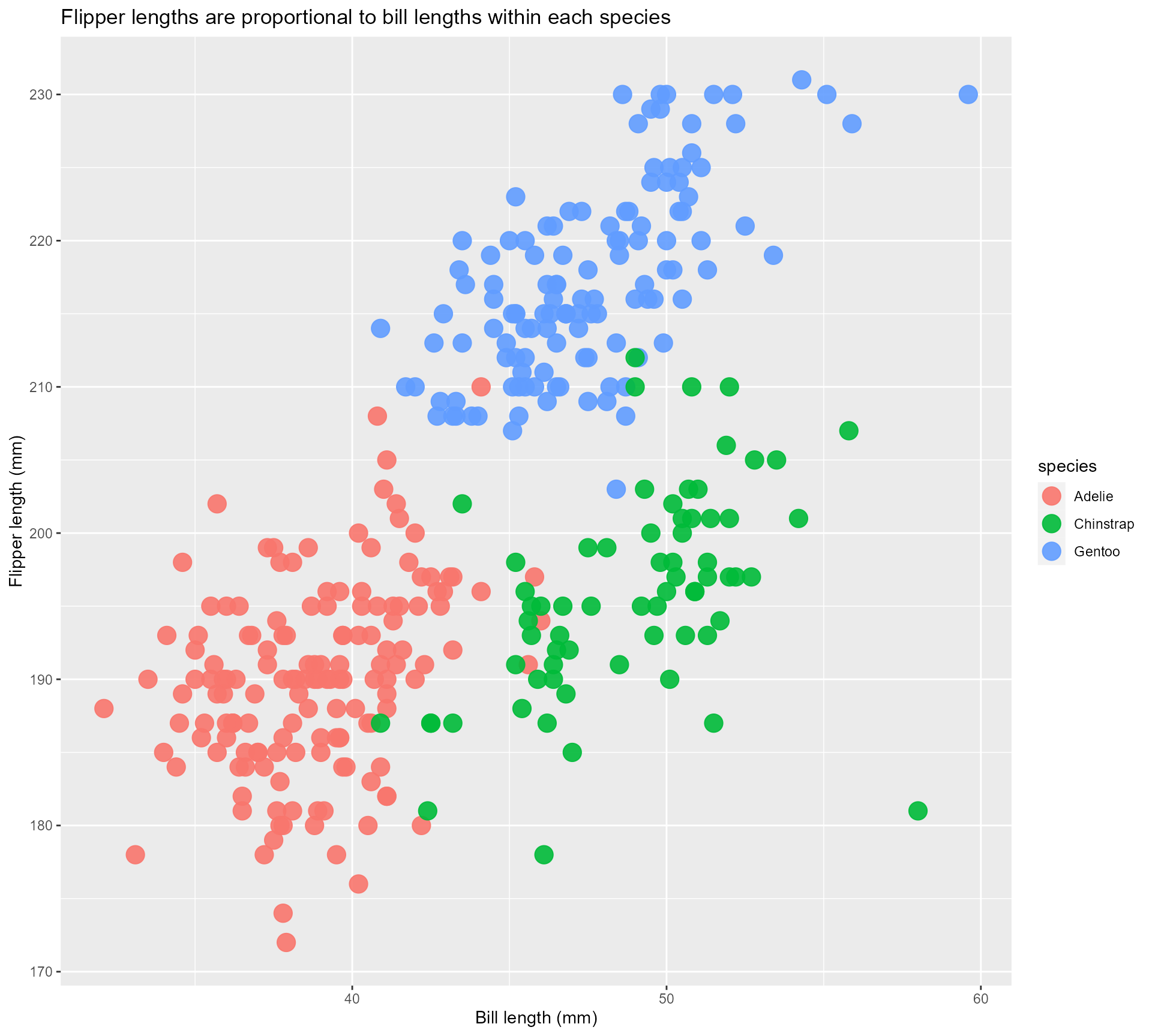
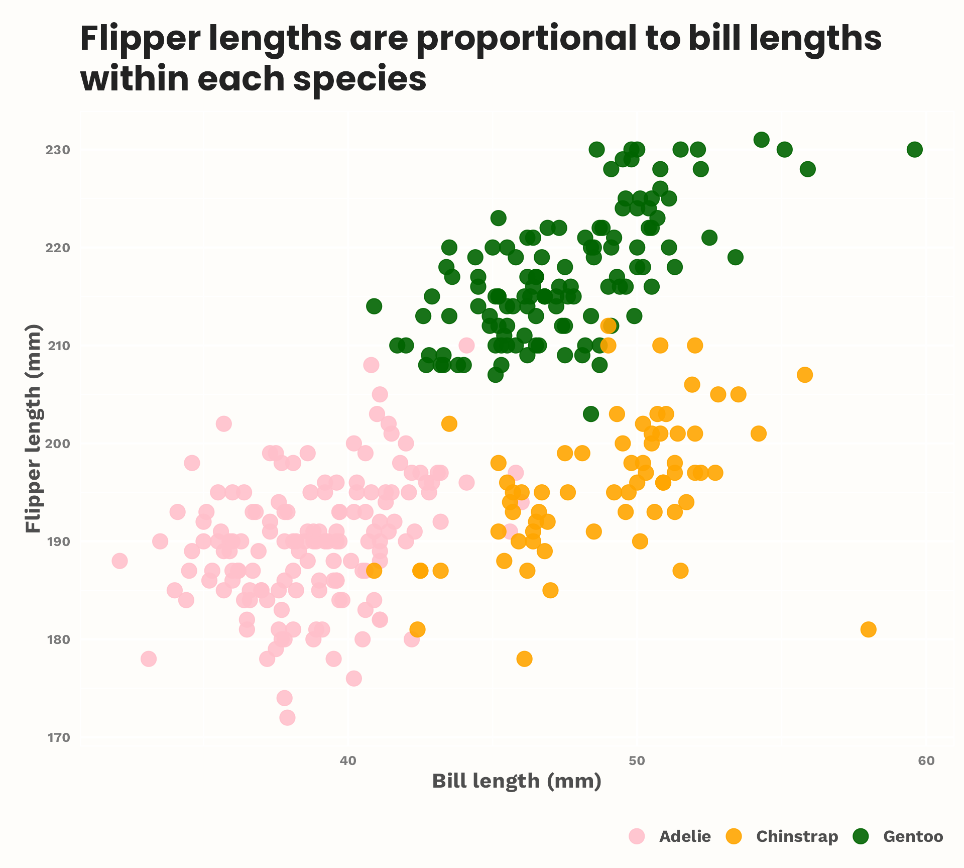
labs(title = "Flipper lengths are proportional to bill lengths within each species",
x = "Bill length (mm)",
y = "Flipper length (mm)") +
theme_minimal() +
scale_colour_manual(values = c("pink",
"orange",
"darkgreen"))
Let’s add some style!
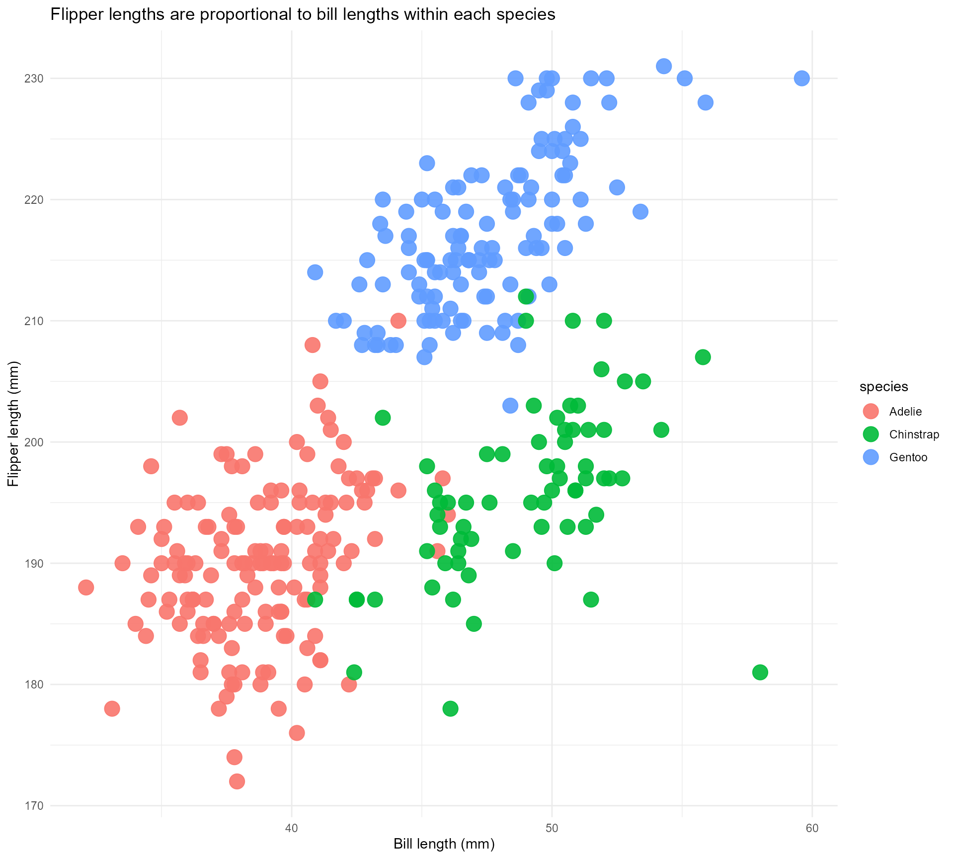
Change the colours - wait a minute…
head(palmerpenguins::penguins, 200) |>
  ggplot() +
  geom_point(aes(x = bill_length_mm,
                 y = flipper_length_mm,
                 colour = species),
             size = 5,
             alpha = 0.9) +
  labs(title = "Flipper lengths are proportional to bill lengths within each species",
       x = "Bill length (mm)",
       y = "Flipper length (mm)") +
  theme_minimal() +
  scale_colour_manual(values = c("pink",
                                 "orange",
                                 "darkgreen"))
Let’s add some style!
Mini tip #1: Named vectors for colours!
penguin_colours <- c(Adelie = "pink",
                     Chinstrap = "orange",
                     Gentoo = "darkgreen")

palmerpenguins::penguins |>
  ggplot() +
  geom_point(aes(x = bill_length_mm,
                 y = flipper_length_mm,
                 colour = species),
             size = 5,
             alpha = 0.9) +
  labs(title = "Flipper lengths are proportional to bill lengths within each species",
       x = "Bill length (mm)",
       y = "Flipper length (mm)") +
  theme_minimal() +
  scale_colour_manual(values = penguin_colours)
Let’s add some style!
Mini tip #1: Named vectors for colours!
penguin_colours <- c(Adelie = "pink",
                     Chinstrap = "orange",
                     Gentoo = "darkgreen")

head(palmerpenguins::penguins, 200) |>
  ggplot() +
  geom_point(aes(x = bill_length_mm,
                 y = flipper_length_mm,
                 colour = species),
             size = 5,
             alpha = 0.9) +
  labs(title = "Flipper lengths are proportional to bill lengths within each species",
       x = "Bill length (mm)",
       y = "Flipper length (mm)") +
  theme_minimal() +
  scale_colour_manual(values = penguin_colours)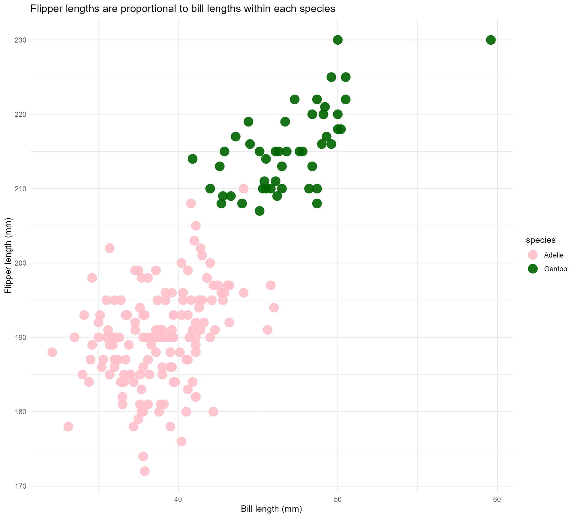
Let’s add some style!
Mini tip #2: Invest in your own custom theme
penguin_colours <- c(Adelie = "pink",
                     Chinstrap = "orange",
                     Gentoo = "darkgreen")

palmerpenguins::penguins |>
  ggplot() +
  geom_point(aes(x = bill_length_mm,
                 y = flipper_length_mm,
                 colour = species),
             size = 5,
             alpha = 0.9) +
  labs(title = "Flipper lengths are proportional to bill lengths within each species",
       x = "Bill length (mm)",
       y = "Flipper length (mm)",
       colour = "") +
  theme_dt_demo() +
  scale_colour_manual(values = penguin_colours)
Let’s add some style!
Mini tip #2: Invest in your own custom theme with relative text sizes
penguin_colours <- c(Adelie = "pink",
                     Chinstrap = "orange",
                     Gentoo = "darkgreen")

palmerpenguins::penguins |>
  ggplot() +
  geom_point(aes(x = bill_length_mm,
                 y = flipper_length_mm,
                 colour = species),
             size = 5,
             alpha = 0.9) +
  labs(title = "Flipper lengths are proportional to bill lengths within each species",
       x = "Bill length (mm)",
       y = "Flipper length (mm)",
       colour = "") +
  theme_dt_demo(base_size = 16) +
  scale_colour_manual(values = penguin_colours)
Let’s add some annotations
I ❤️ {ggtext}
mean_x_y <- palmerpenguins::penguins |>
  group_by(species) |>
  summarise(mean_x = mean(bill_length_mm, na.rm = TRUE),
            mean_y = mean(flipper_length_mm, na.rm = TRUE))

palmerpenguins::penguins |>
  ggplot() +
  geom_point(aes(x = bill_length_mm,
                 y = flipper_length_mm,
                 colour = species),
             size = 5,
             alpha = 0.9) +
  ggtext::geom_textbox(data = mean_x_y,
                       aes(x = mean_x,
                           y = mean_y,
                           label = species),
                       size = 7) +
  labs(title = "Flipper lengths are proportional to bill lengths within each species",
       x = "Bill length (mm)",
       y = "Flipper length (mm)",
       colour = "") +
  theme_dt_demo(16) +
  scale_colour_manual(values = penguin_colours)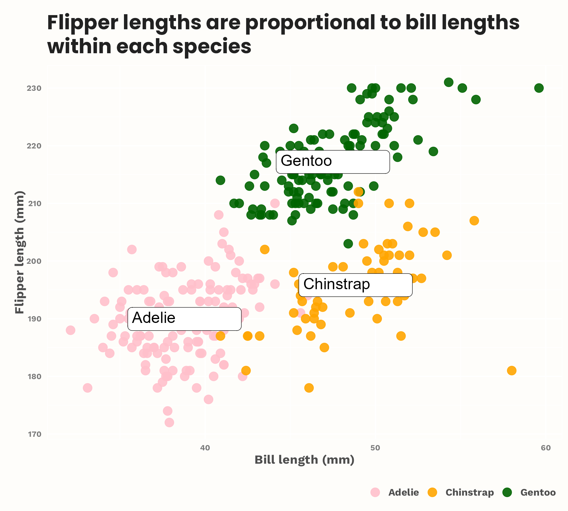
Let’s add some annotations
I ❤️ {ggtext}
mean_x_y <- palmerpenguins::penguins |>
  group_by(species) |>
  summarise(mean_x = mean(bill_length_mm, na.rm = TRUE),
            mean_y = mean(flipper_length_mm, na.rm = TRUE),
            count = length(species))

palmerpenguins::penguins |>
  ggplot() +
  geom_point(aes(x = bill_length_mm,
                 y = flipper_length_mm,
                 colour = species),
             size = 5,
             alpha = 0.9,
             show.legend = FALSE) +
  ggtext::geom_textbox(data = mean_x_y,
                       aes(x = mean_x,
                           y = mean_y,
                           label = paste0("**", species, "**",
                                          "<br>N = ", count)),
                       size = 7) +
  labs(title = "Flipper lengths are proportional to bill lengths within each species",
       x = "Bill length (mm)",
       y = "Flipper length (mm)",
       colour = "") +
  theme_dt_demo(16) +
  scale_colour_manual(values = penguin_colours)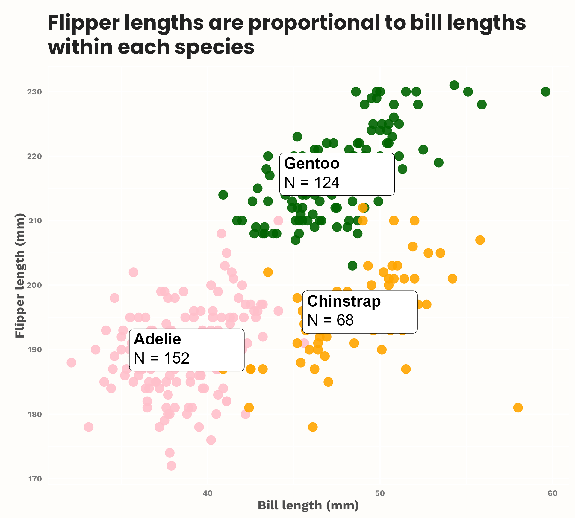
Let’s add some annotations
I ❤️ {ggtext}
mean_x_y <- palmerpenguins::penguins |>
group_by(species) |>
summarise(mean_x = mean(bill_length_mm, na.rm = TRUE),
mean_y = mean(flipper_length_mm, na.rm = TRUE),
mean_weight = mean(body_mass_g, na.rm = TRUE),
count = length(species))
palmerpenguins::penguins |>
ggplot() +
geom_point(aes(x = bill_length_mm,
y = flipper_length_mm,
colour = species),
size = 5,
alpha = 0.9,
show.legend = FALSE) +
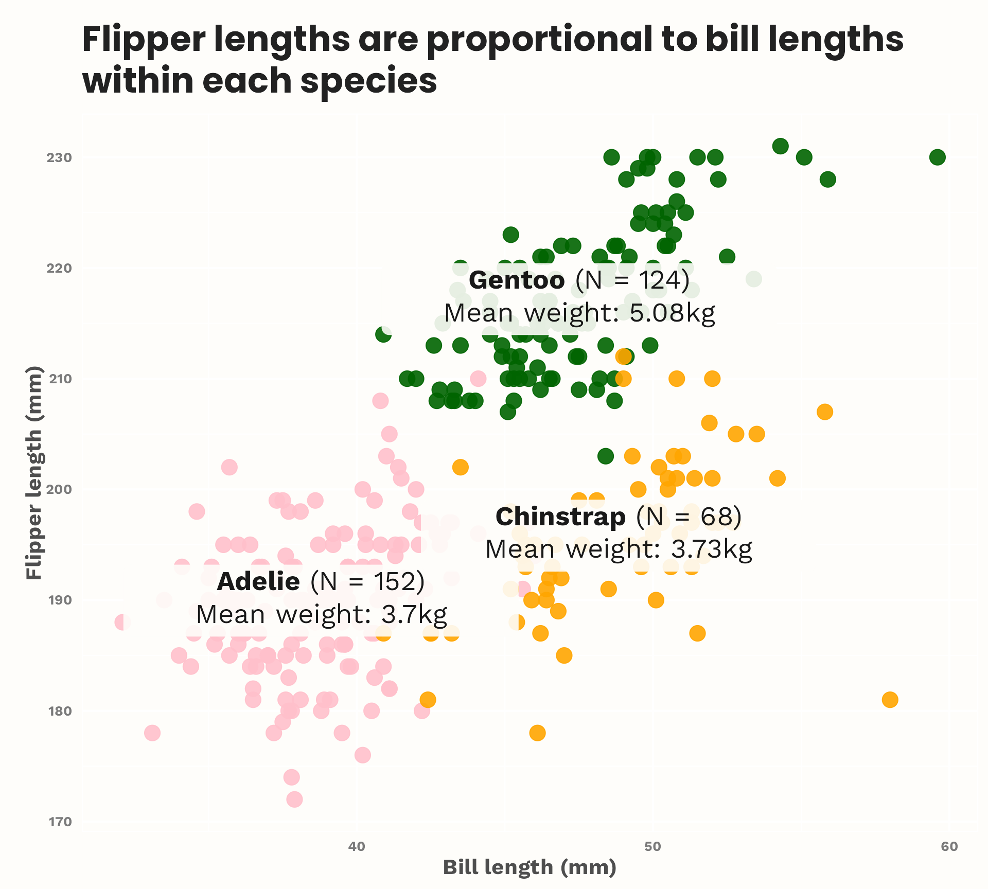
ggtext::geom_textbox(data = mean_x_y,
aes(x = mean_x,
y = mean_y,
label = paste0("**", species, "**",
" (N = ", count, ")",
"<br>Mean weight: ", janitor::round_half_up(mean_weight/1000, 2), "kg")),
size = 7) +
labs(title = "Flipper lengths are proportional to bill lengths within each species",
x = "Bill length (mm)",
y = "Flipper length (mm)",
colour = "") +
theme_dt_demo(16) +
scale_colour_manual(values = penguin_colours)
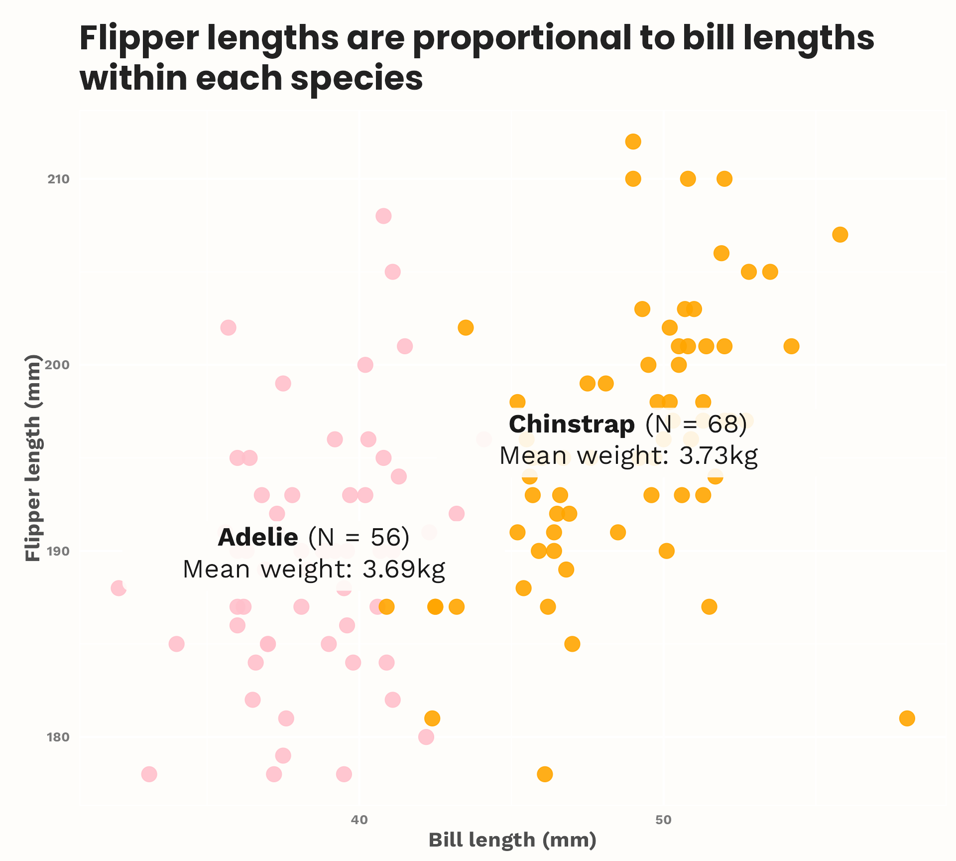
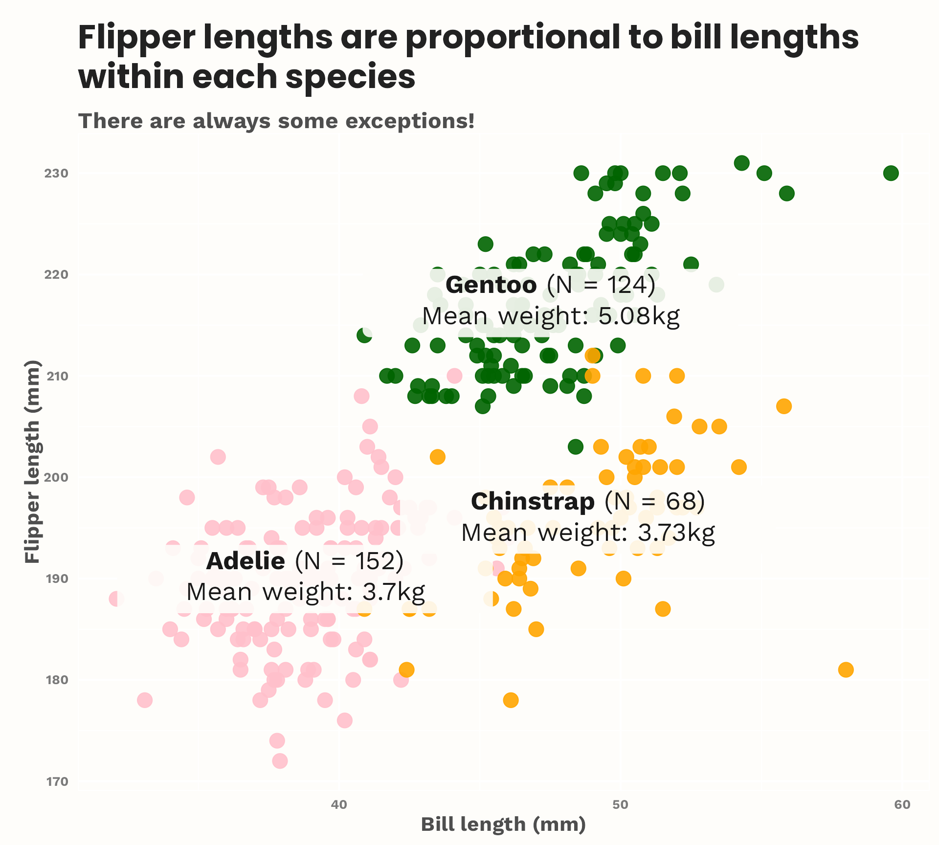
Let’s add some annotations
I ❤️ {ggtext}
mean_x_y <- palmerpenguins::penguins |>
  group_by(species) |>
  summarise(mean_x = mean(bill_length_mm, na.rm = TRUE),
            mean_y = mean(flipper_length_mm, na.rm = TRUE),
            mean_weight = mean(body_mass_g, na.rm = TRUE),
            count = length(species))

palmerpenguins::penguins |>
  ggplot() +
  geom_point(aes(x = bill_length_mm,
                 y = flipper_length_mm,
                 colour = species,
                 size = body_mass_g),
             size = 5,
             alpha = 0.9,
             show.legend = FALSE) +
  ggtext::geom_textbox(data = mean_x_y,
                       aes(x = mean_x,
                           y = mean_y,
                           label = paste0("**", species, "**",
                                          " (N = ", count, ")",
                                          "<br>Mean weight: ", janitor::round_half_up(mean_weight/1000, 2), "kg")),
                       size = 7,
                       family = "Work Sans",
                       width = unit(20, "lines"),
                       fill = "#FEFDFA",
                       box.colour = NA,
                       alpha = 0.9,
                       halign = 0.5) +
  labs(title = "Flipper lengths are proportional to bill lengths within each species",
       x = "Bill length (mm)",
       y = "Flipper length (mm)",
       colour = "") +
  theme_dt_demo() +
  scale_colour_manual(values = penguin_colours)
From basic to styled and annotated
From basic to styled and annotated
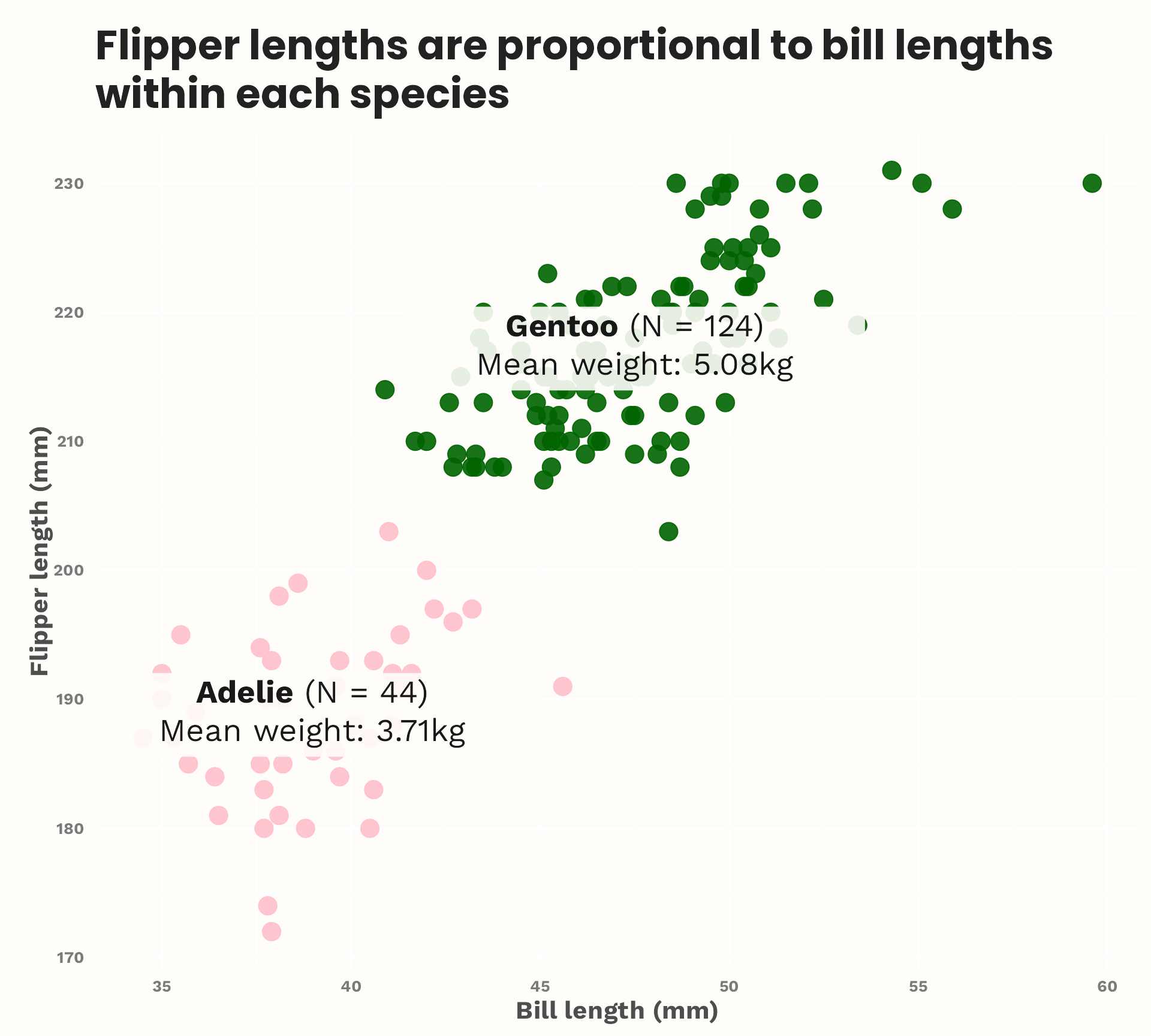
Parameterisation #1: Different data
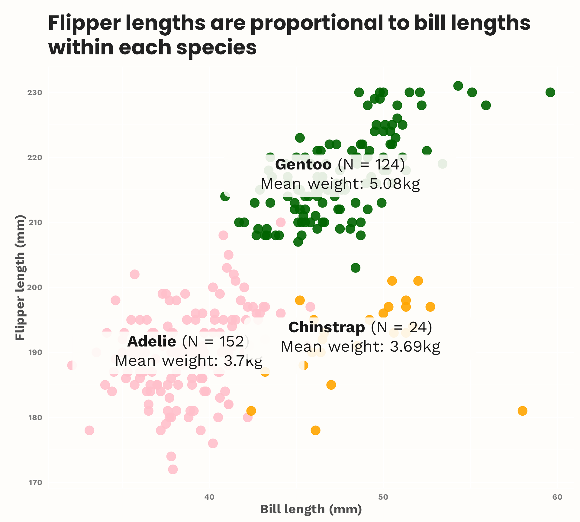
“Oh, I’m sorry, I actually just wanted the first 200 penguins…”
mean_x_y <- head(palmerpenguins::penguins, 200) |>
  group_by(species) |>
  summarise(mean_x = mean(bill_length_mm, na.rm = TRUE),
            mean_y = mean(flipper_length_mm, na.rm = TRUE),
            mean_weight = mean(body_mass_g, na.rm = TRUE),
            count = length(species))

head(palmerpenguins::penguins, 200) |>
  ggplot() +
  geom_point(aes(x = bill_length_mm,
                 y = flipper_length_mm,
                 colour = species,
                 size = body_mass_g),
             size = 5,
             alpha = 0.9,
             show.legend = FALSE) +
  ggtext::geom_textbox(data = mean_x_y,
                       aes(x = mean_x,
                           y = mean_y,
                           label = paste0("**", species, "**",
                                          " (N = ", count, ")",
                                          "<br>Mean weight: ", janitor::round_half_up(mean_weight/1000, 2), "kg")),
                       size = 7,
                       family = "Work Sans",
                       width = unit(20, "lines"),
                       fill = "#FEFDFA",
                       box.colour = NA,
                       alpha = 0.9,
                       halign = 0.5) +
  labs(title = "Flipper lengths are proportional to bill lengths within each species",
       x = "Bill length (mm)",
       y = "Flipper length (mm)",
       colour = "") +
  theme_dt_demo(16) +
  scale_colour_manual(values = penguin_colours)
Parameterisation #1: Different data
“Hmm, wait, could do both, for comparison?”

Parameterisation #1: Different data
“… and could we check with 300 and 400 also?”

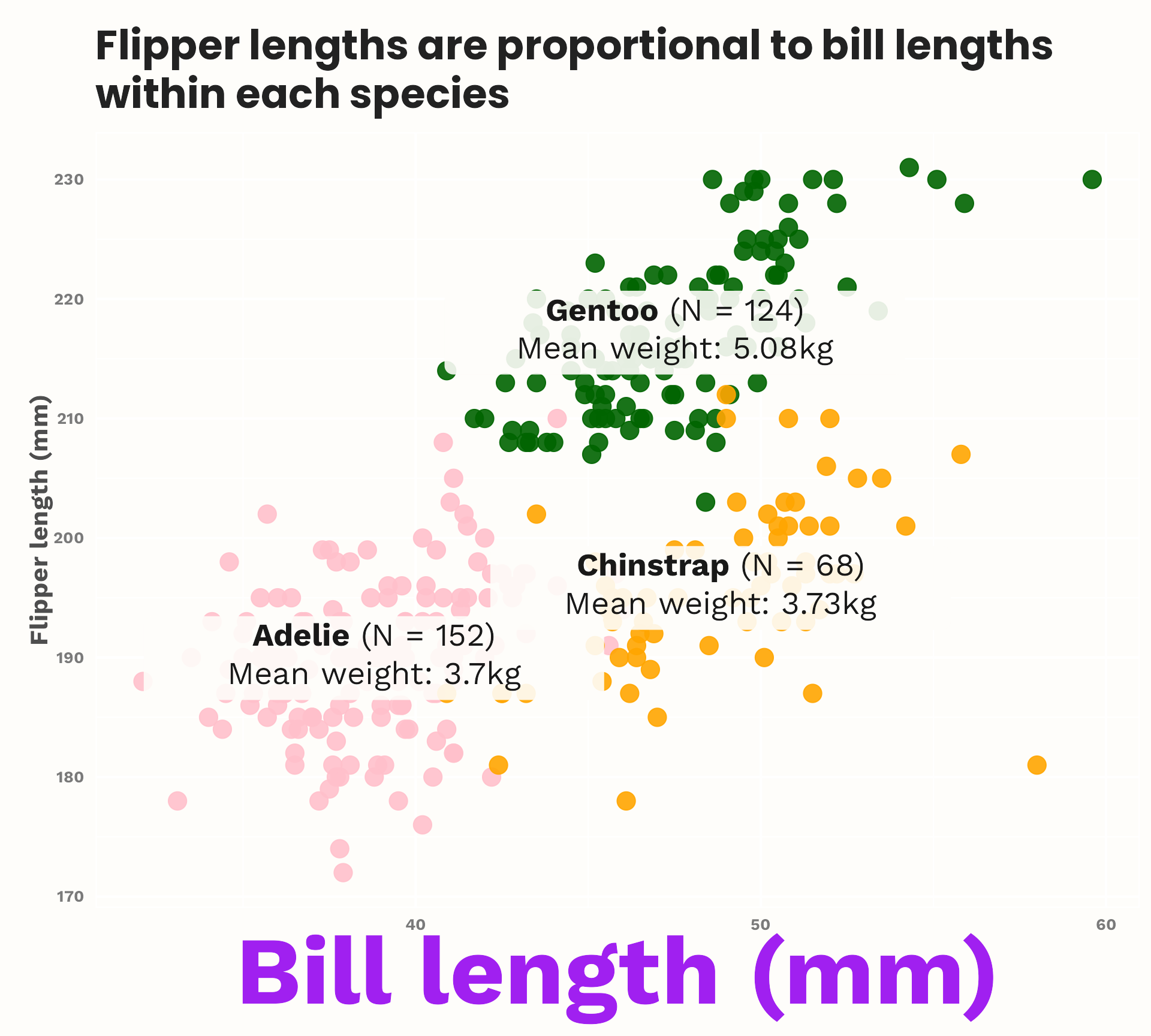
Parameterisation #1: Different data
“I realise the meeting is in 5 minutes, but I really don’t like those fonts and colours… Could you change them?”


Parameterisation #1: Different data
Let’s see the original again…

Parameterisation #1: Different data
And can we do it with just the first 300 and 400 penguins?

Parameterisation #1: Different data
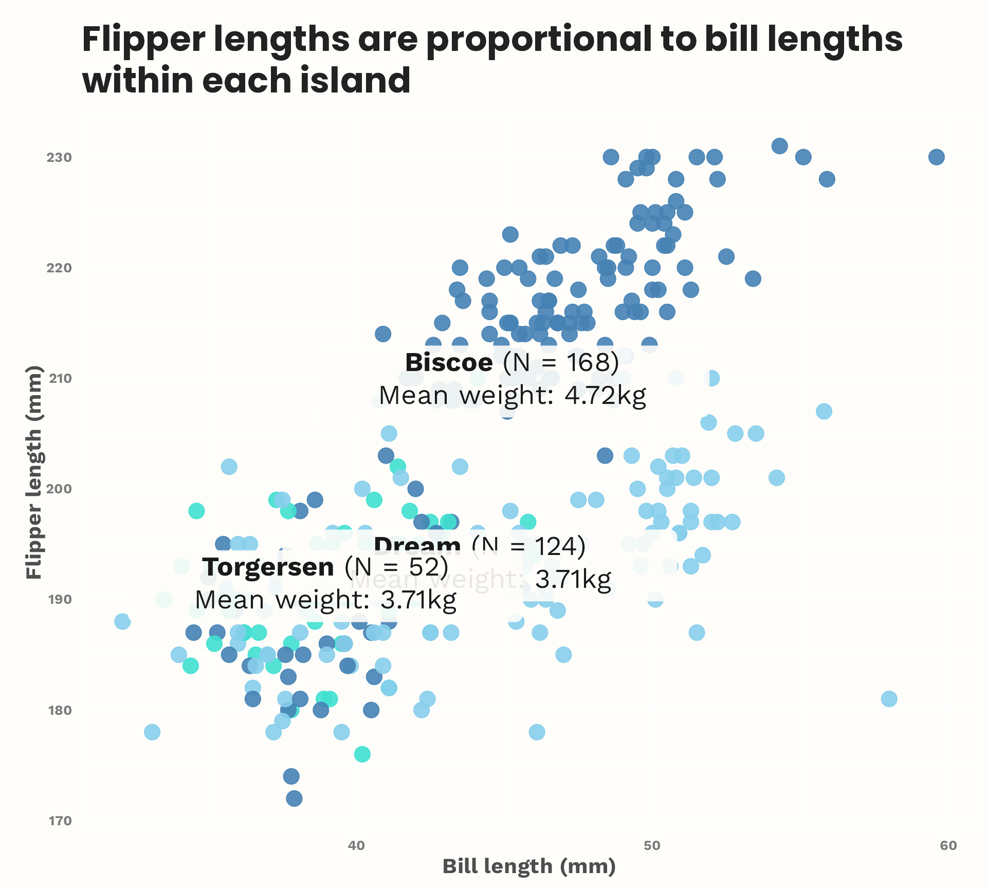
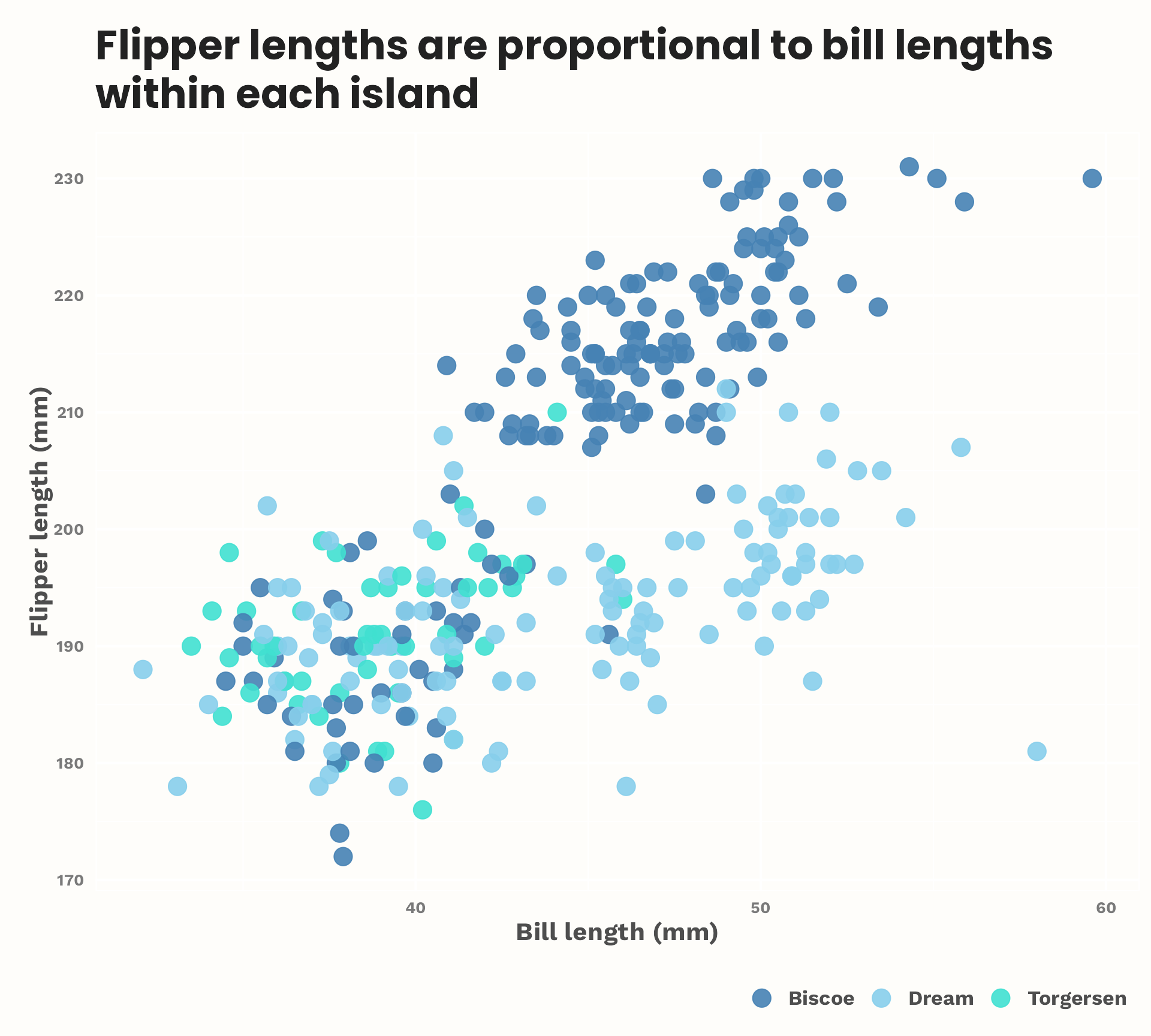
Actually, let’s do it by island…
Parameterisation #2: Different grouping
Rather than grouping by species, can we group by island?

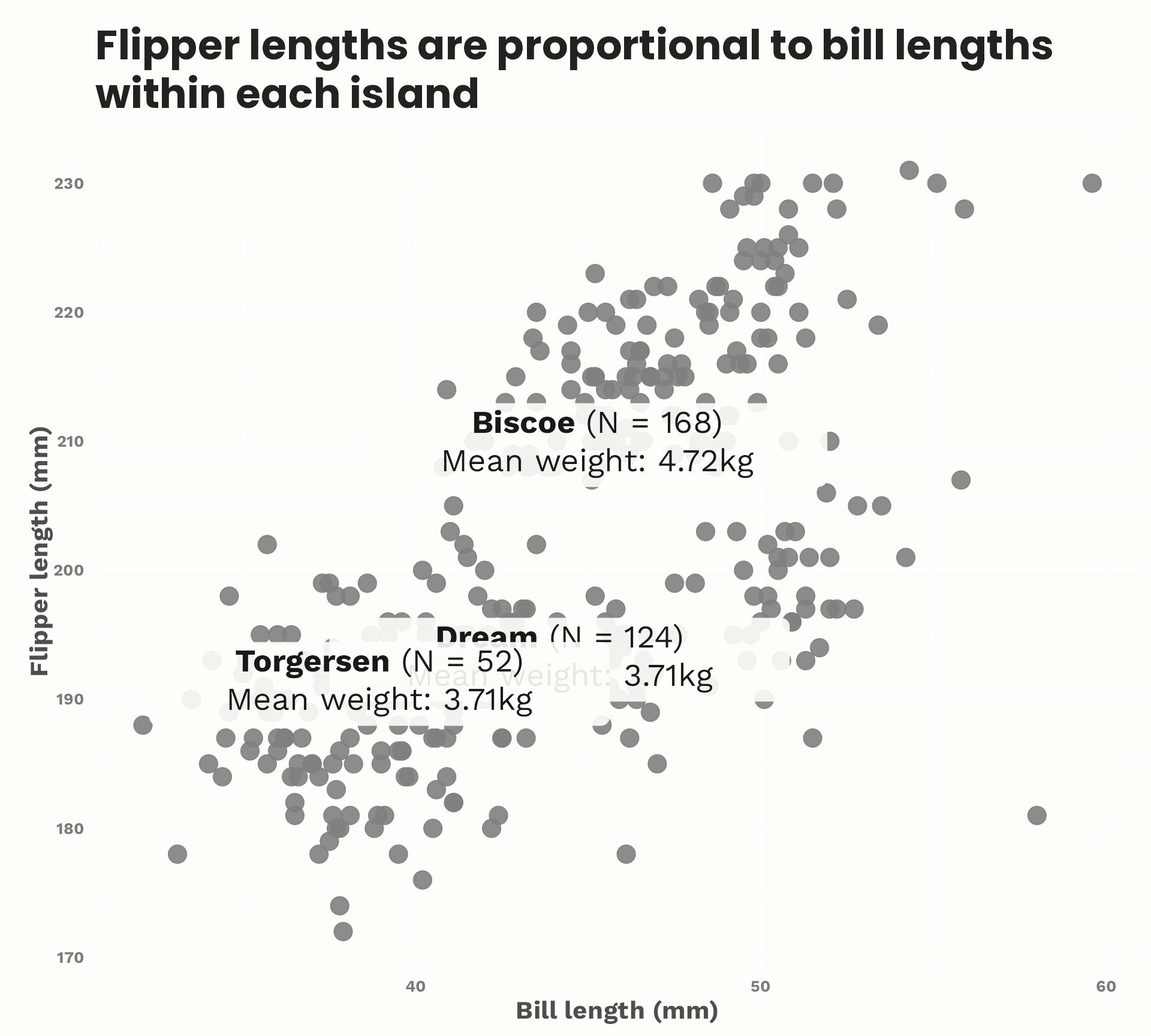
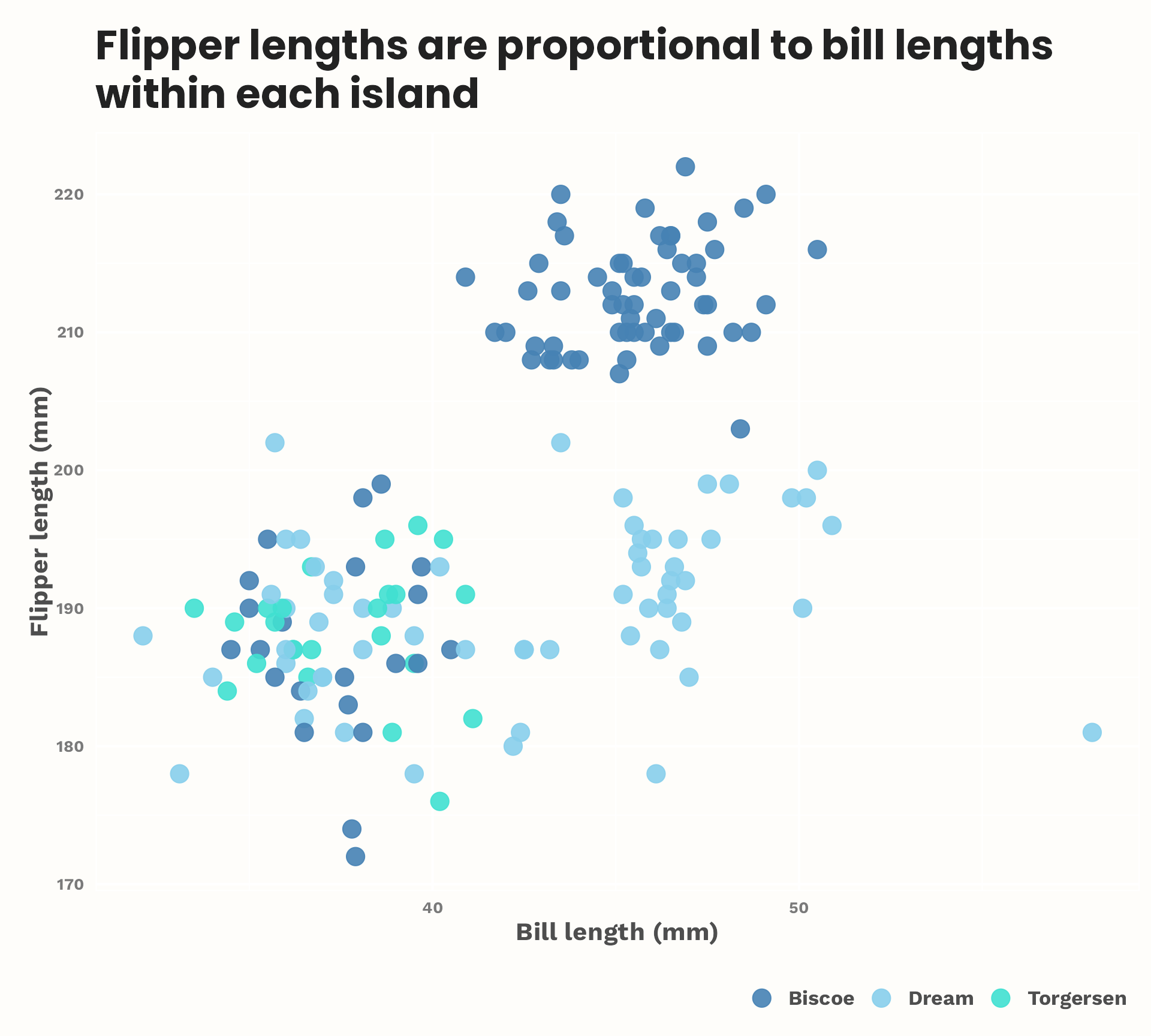
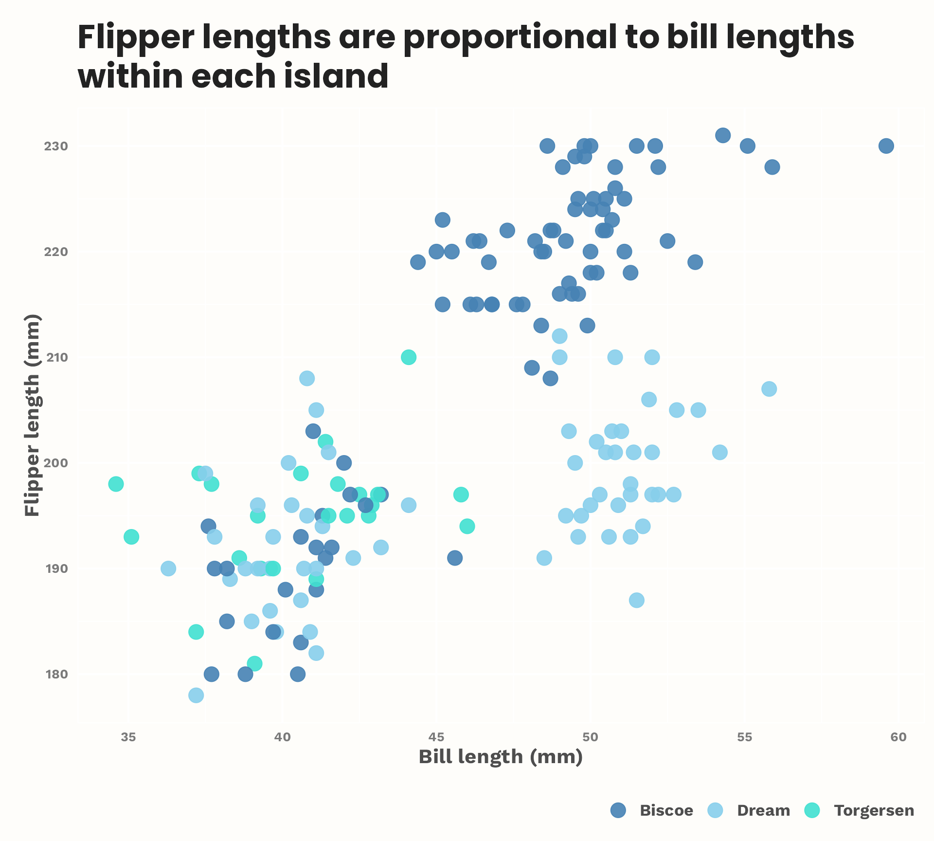
Parameterisation #2: Different grouping
Actually, can we just look at a few different grouping options?
Parameterisation #2: Different grouping
Actually, can we just look at a few different grouping options?

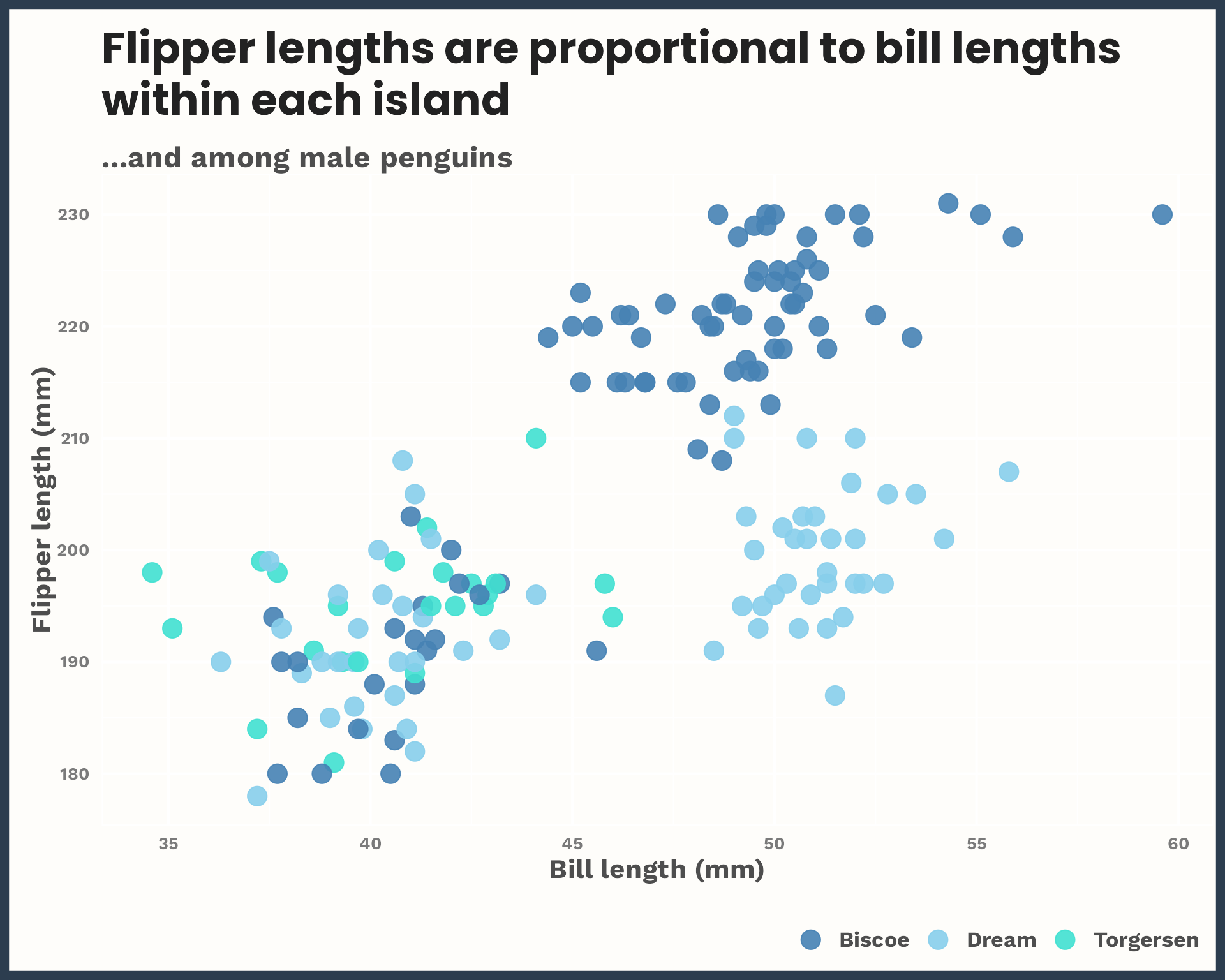
Parameterisation #2: Different grouping
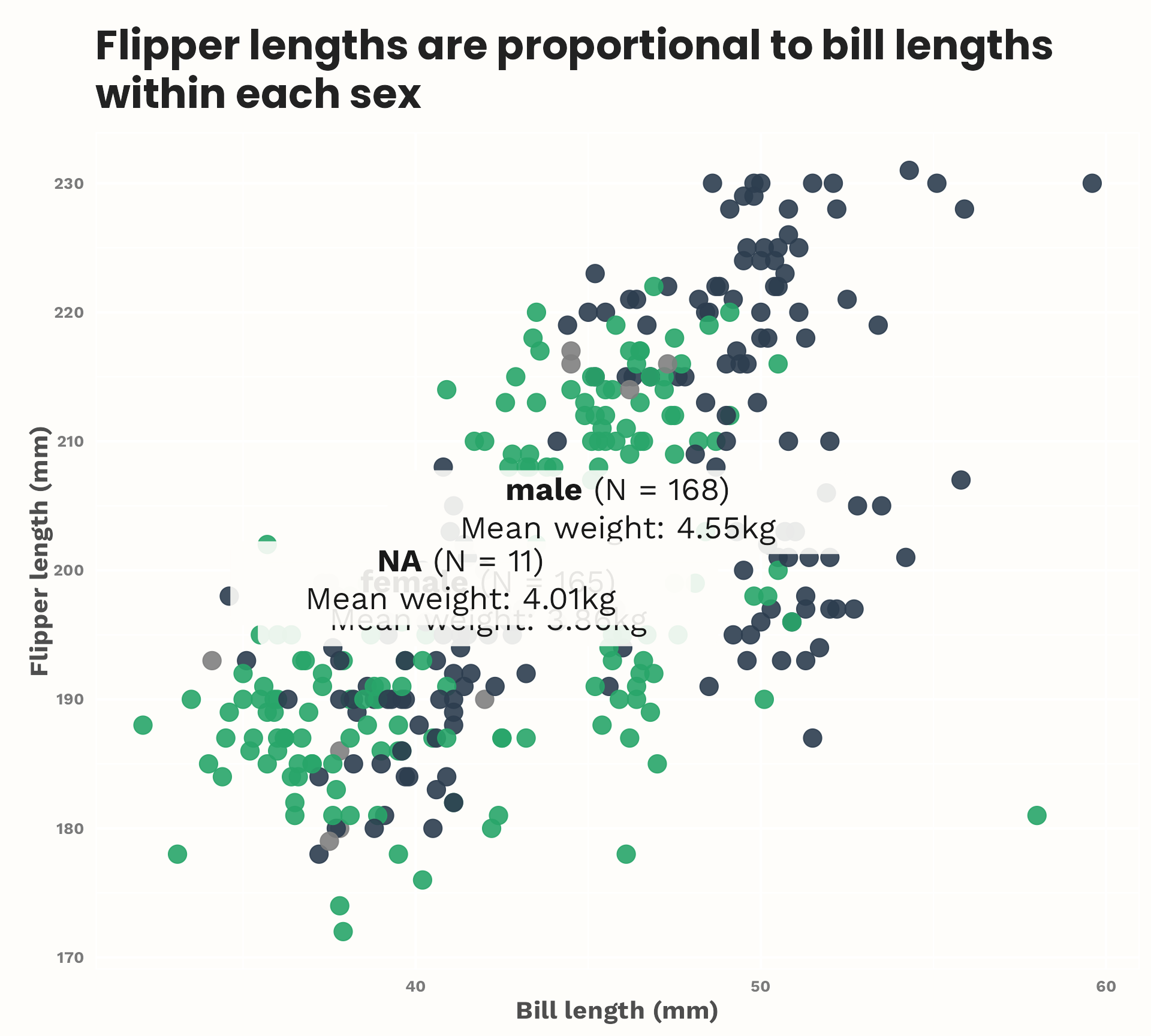
Ok, now split by island within each sex.
Parameterisation #3: Different styling
Switching off the labels

Parameterisation #3: Different styling
Add optional subtitle

Parameterisation #3: Different styling
The magic of ...

Parameterisation #3: Different styling
A more sensible use case…

Give it a go!
cararthompson.com/talks/parameterise
![]()