Make it your own
Tips & trick for stand-out dataviz with R and ggplot2
Cara R Thompson, PhD
26th March 2026
How did I end up here?


How did I end up here?


How did I end up here?
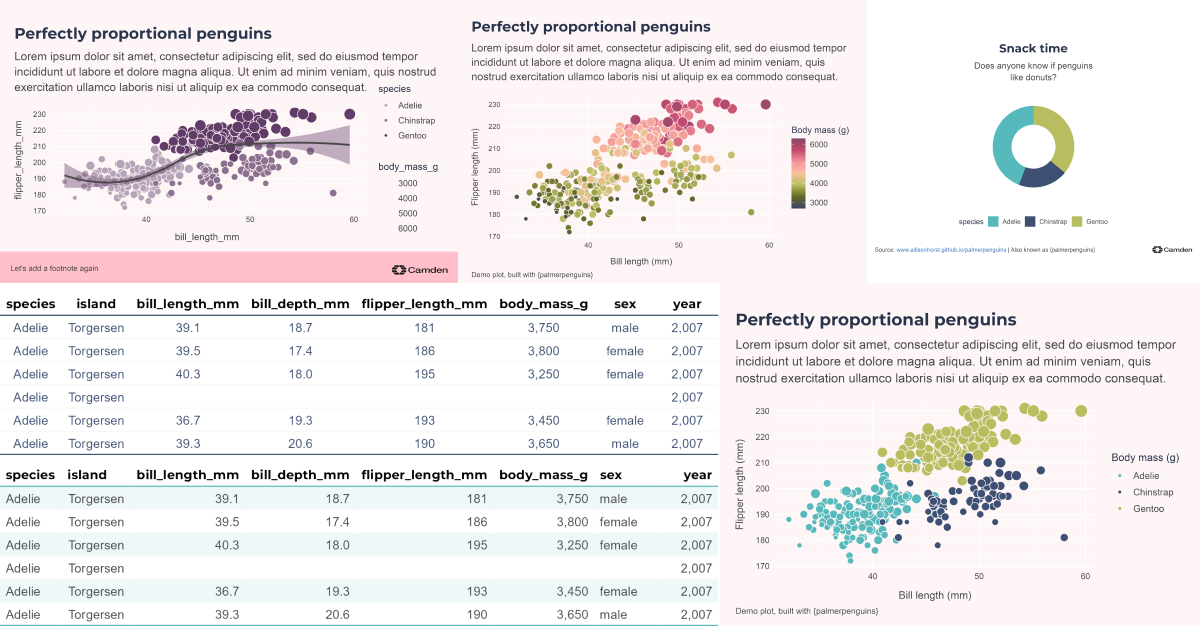
Why dataviz?
“Look, the data really speaks for itself… Here you go!”
Why dataviz better?
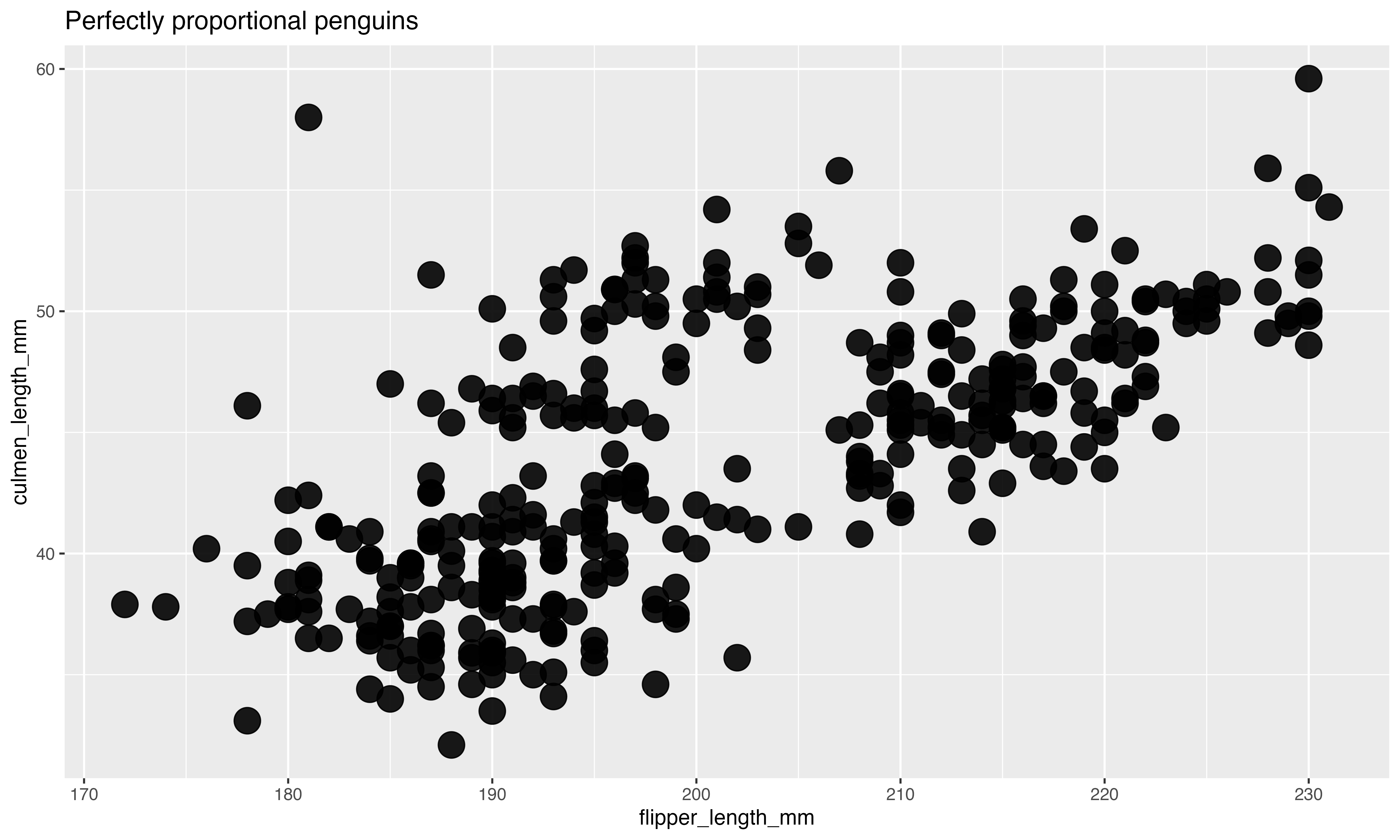
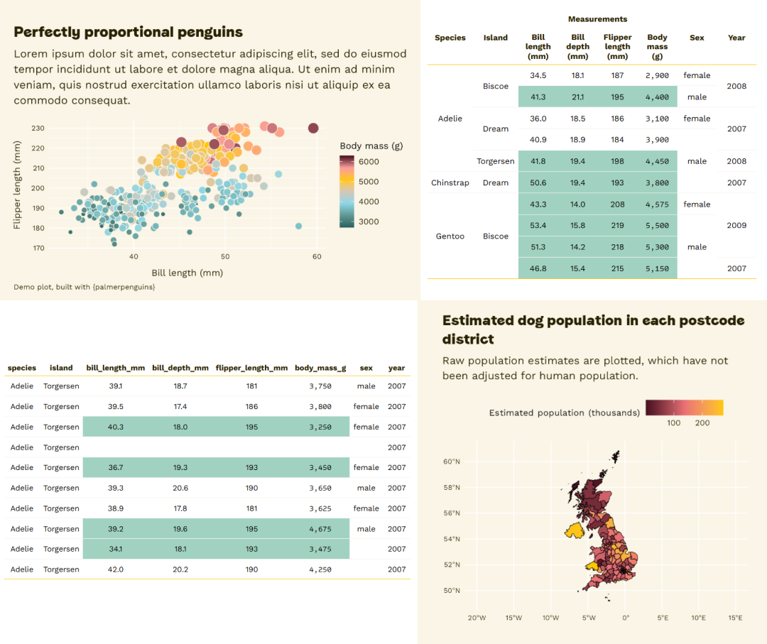
What’s the best way to visualise the story?
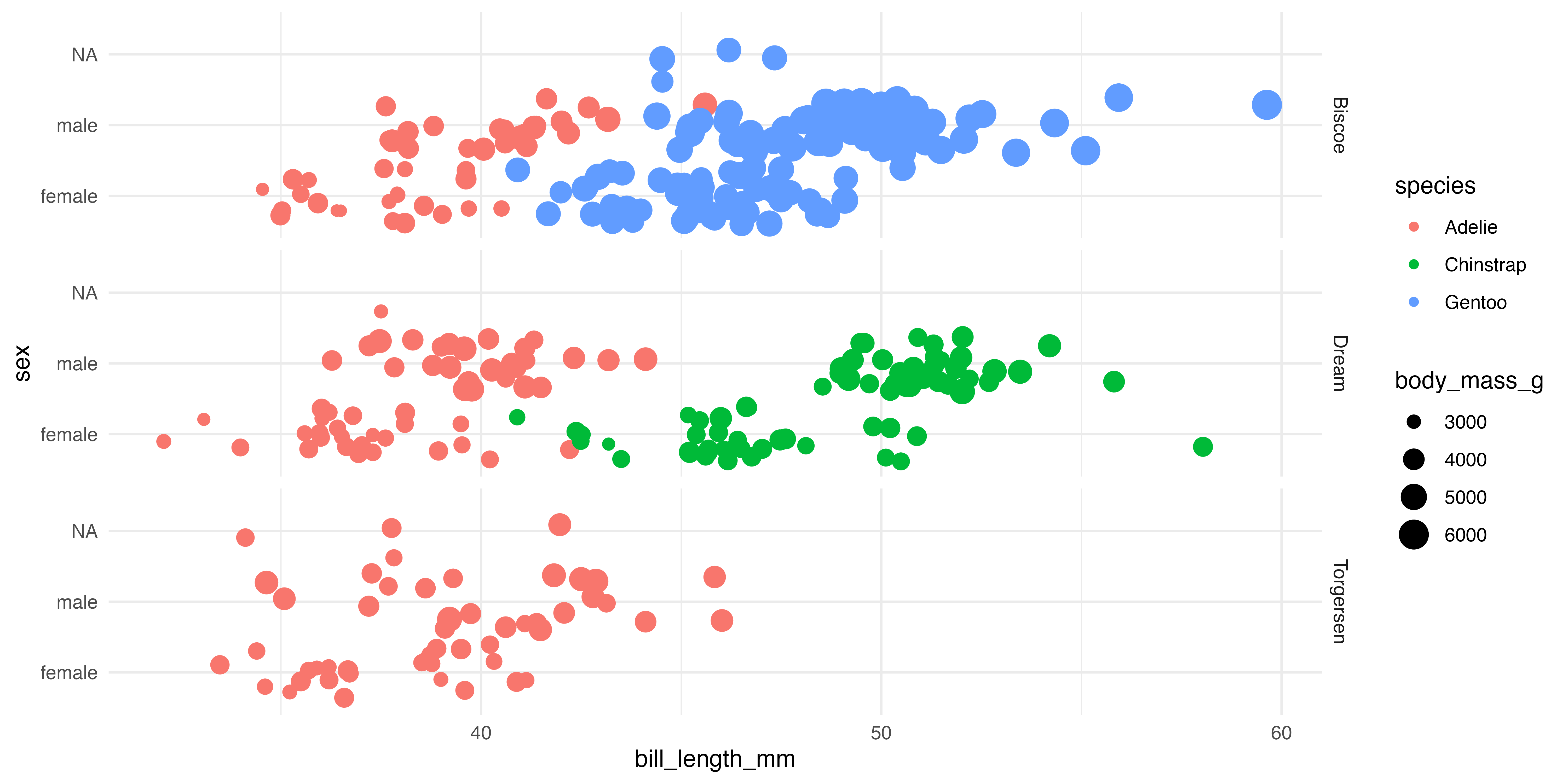
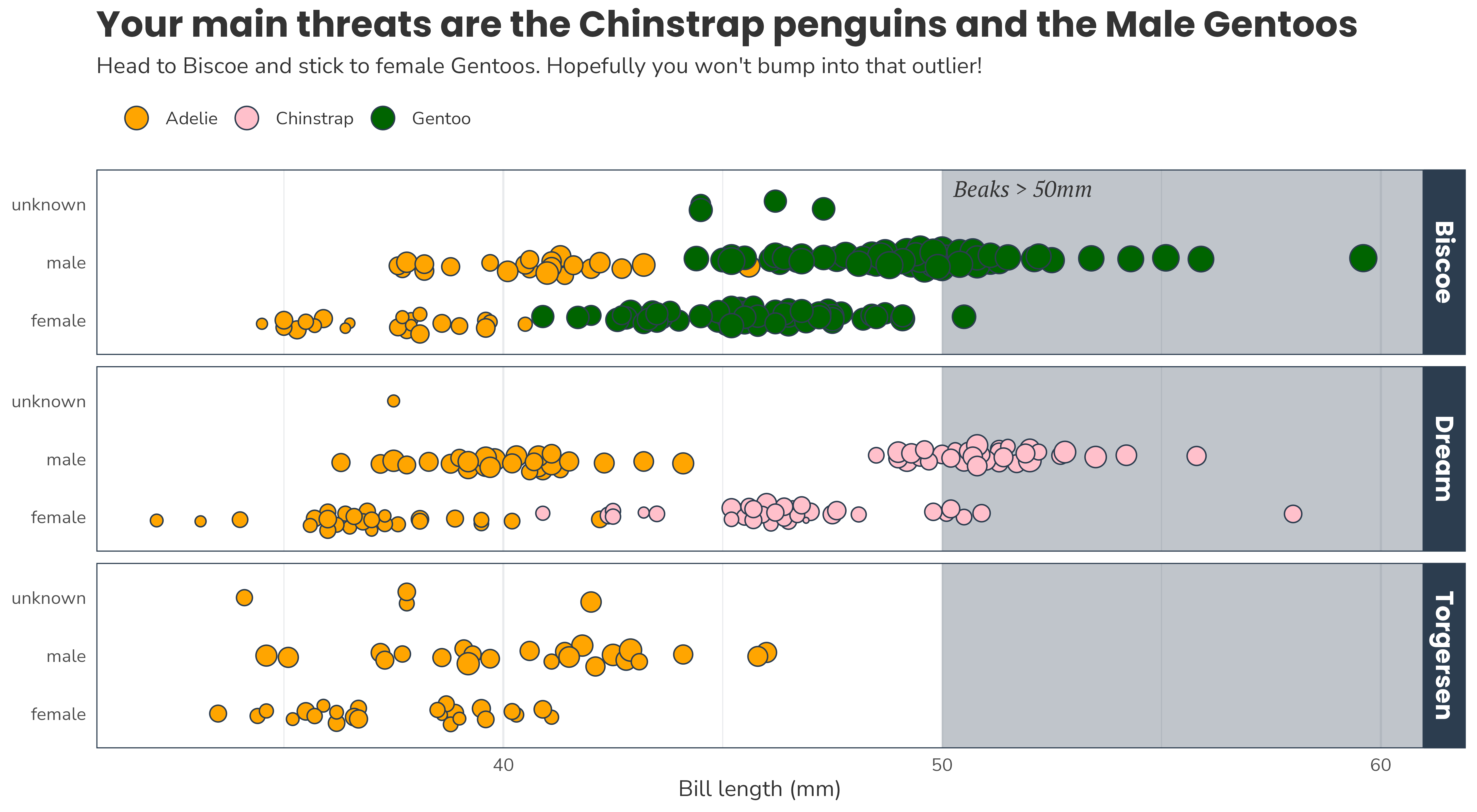
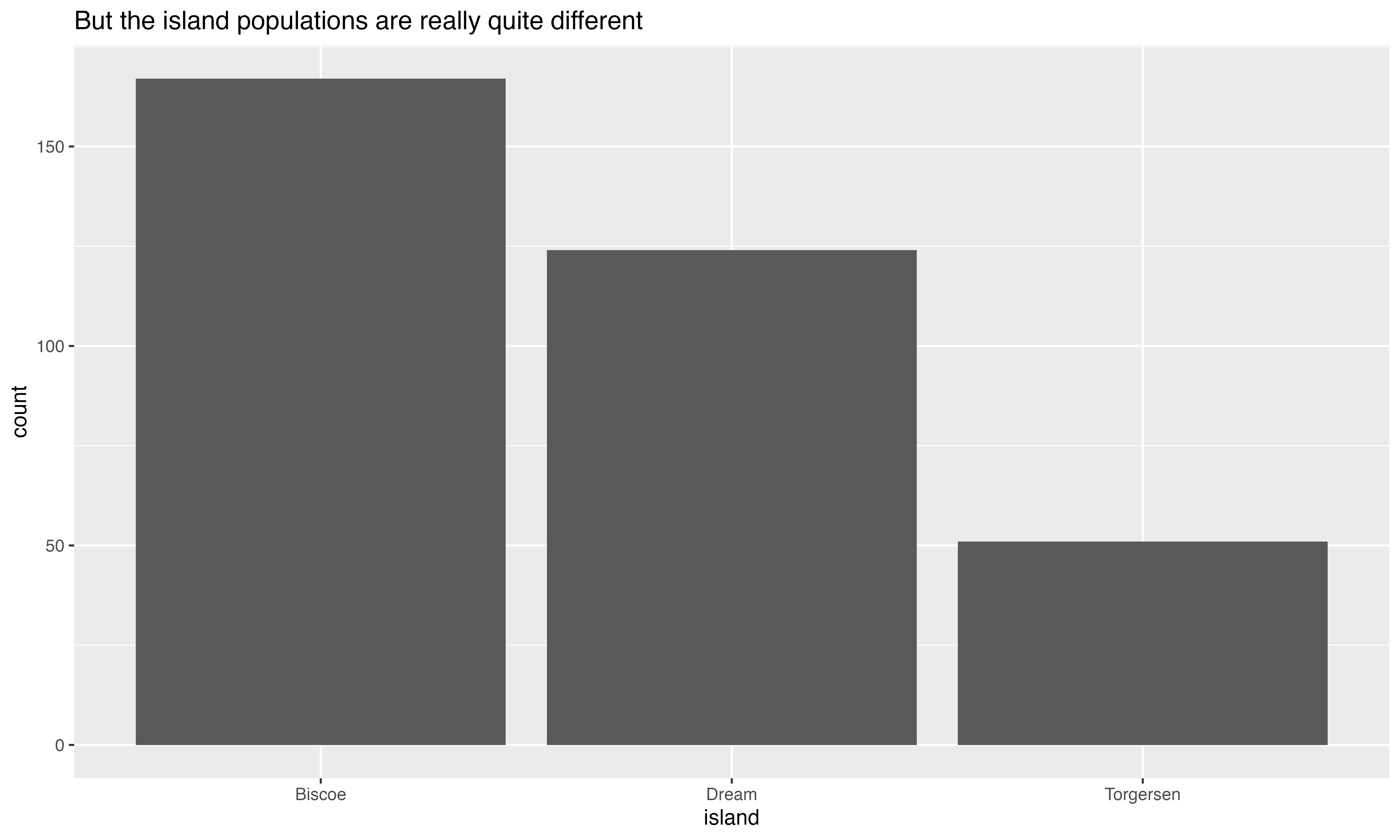
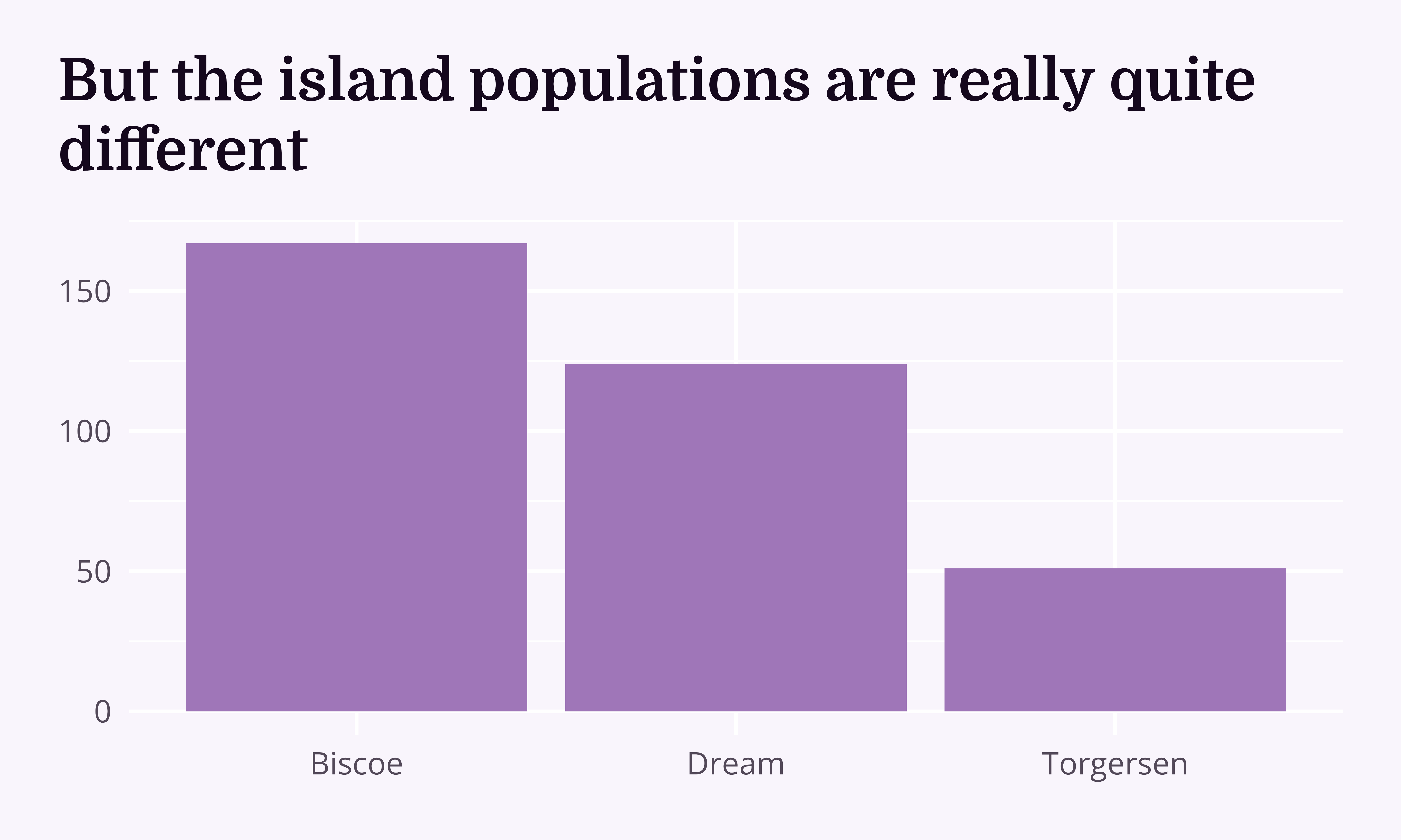
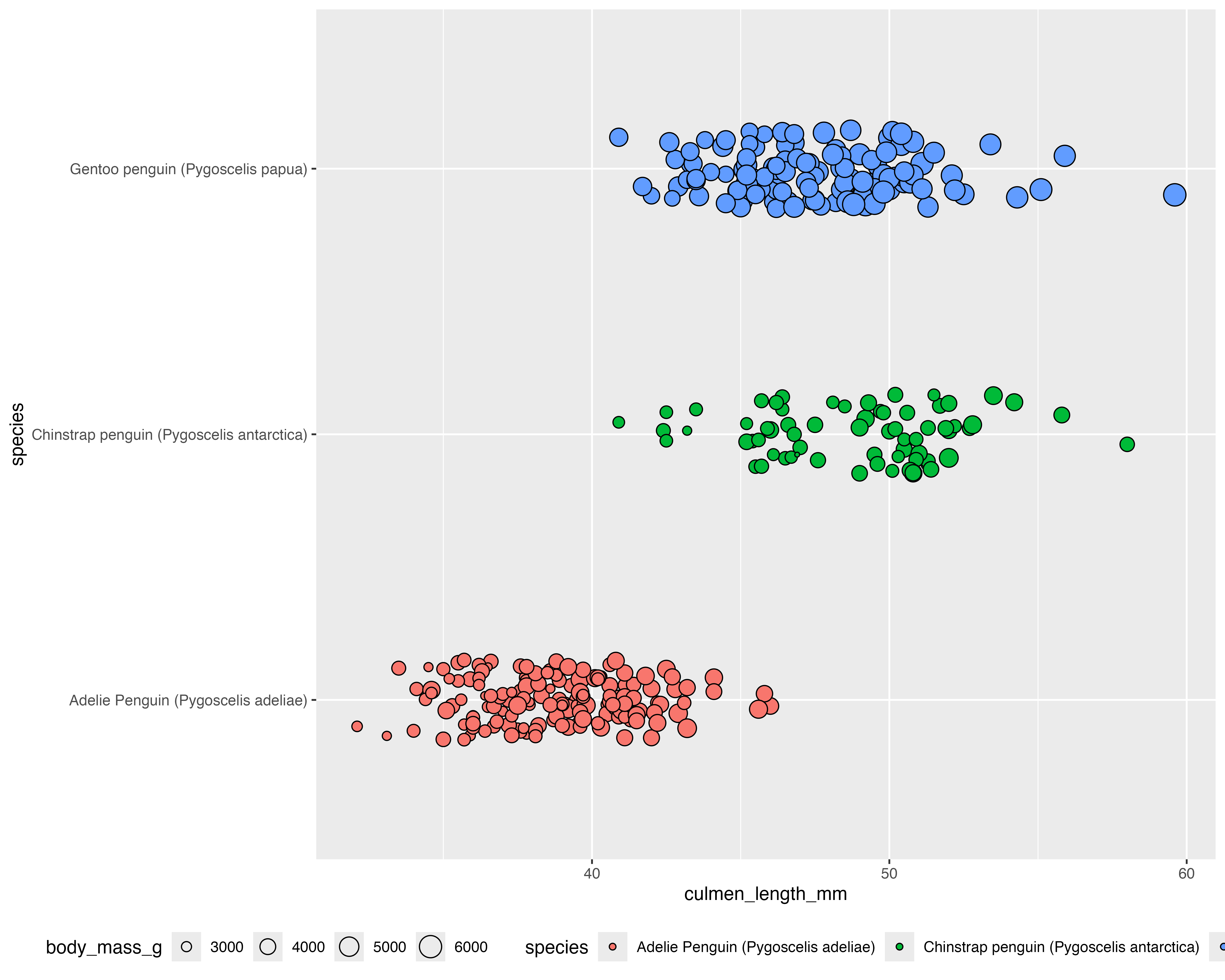
Chester Zoo is welcoming some new penguins from Edinburgh Zoo. The keepers are a bit nervous about how the penguins will all get on.
They get quite competitive within each species about their beak lengths.
If we can see which penguin is which, even better!

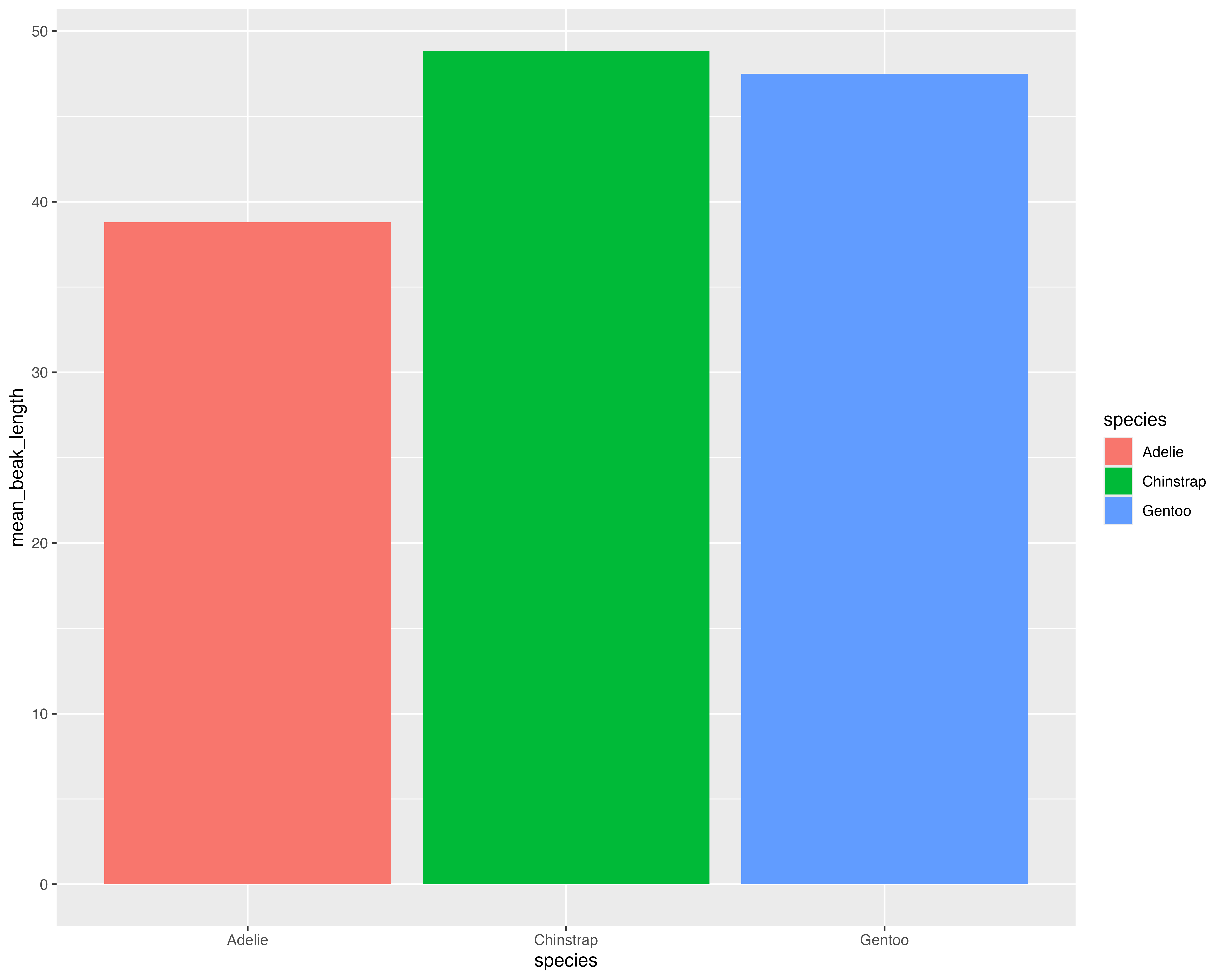
What’s the best way to visualise the story?
- Range of beak (culmen) lengths
- All three species separately
- Some appreciation of outliers
- A way of identifying the penguins
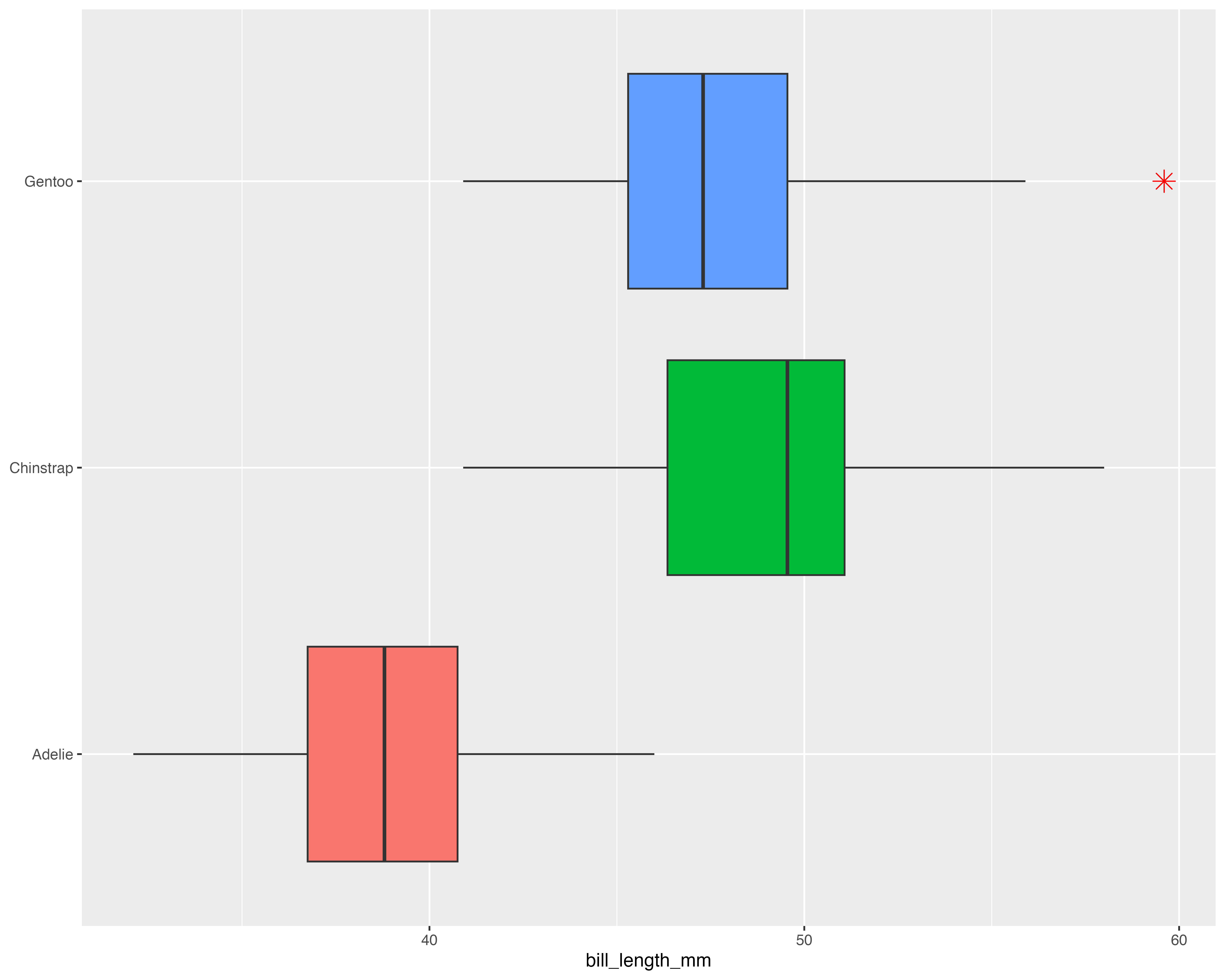
What’s the best way to visualise the story?
What’s the best way to visualise the story?
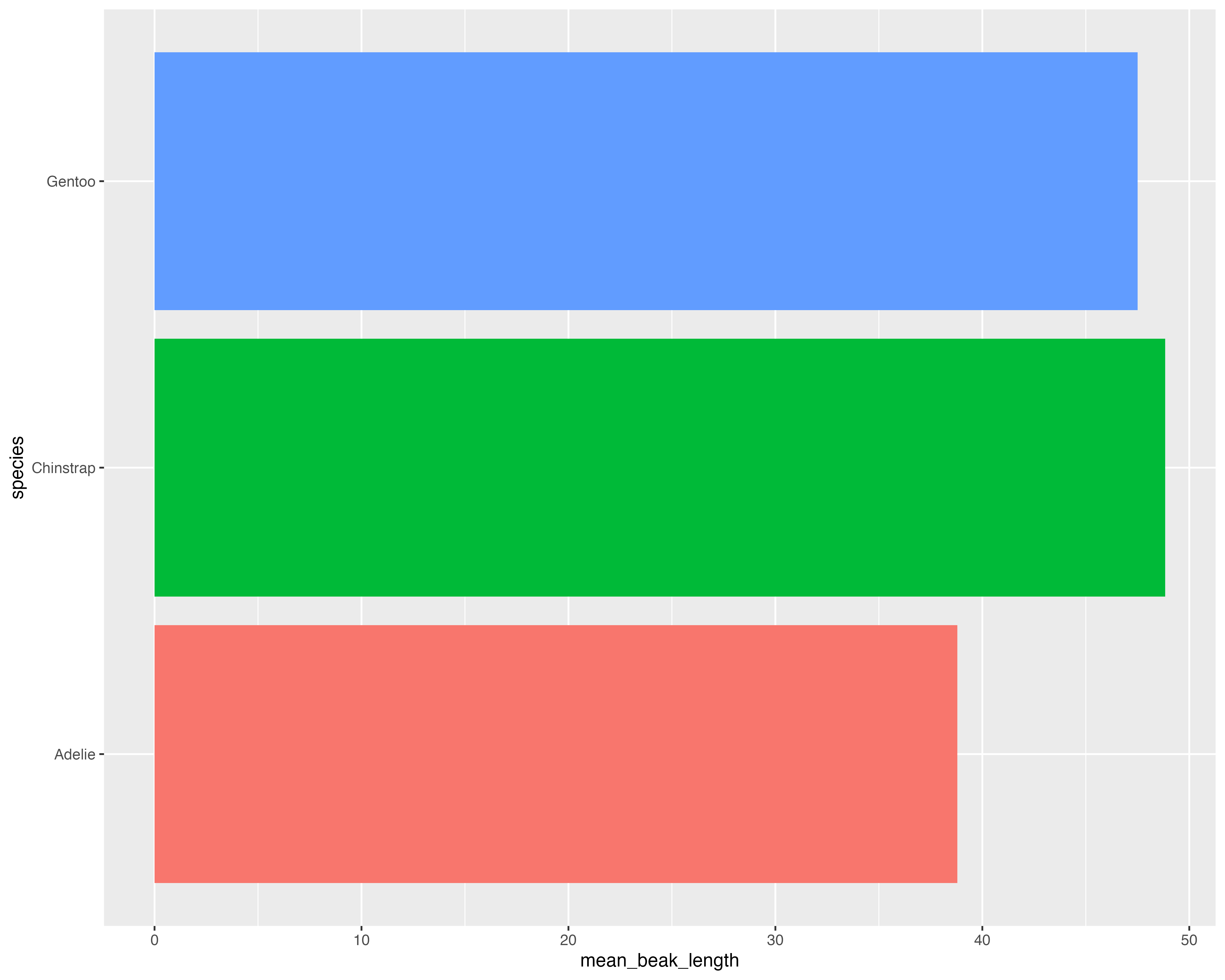
What’s the best way to visualise the story?
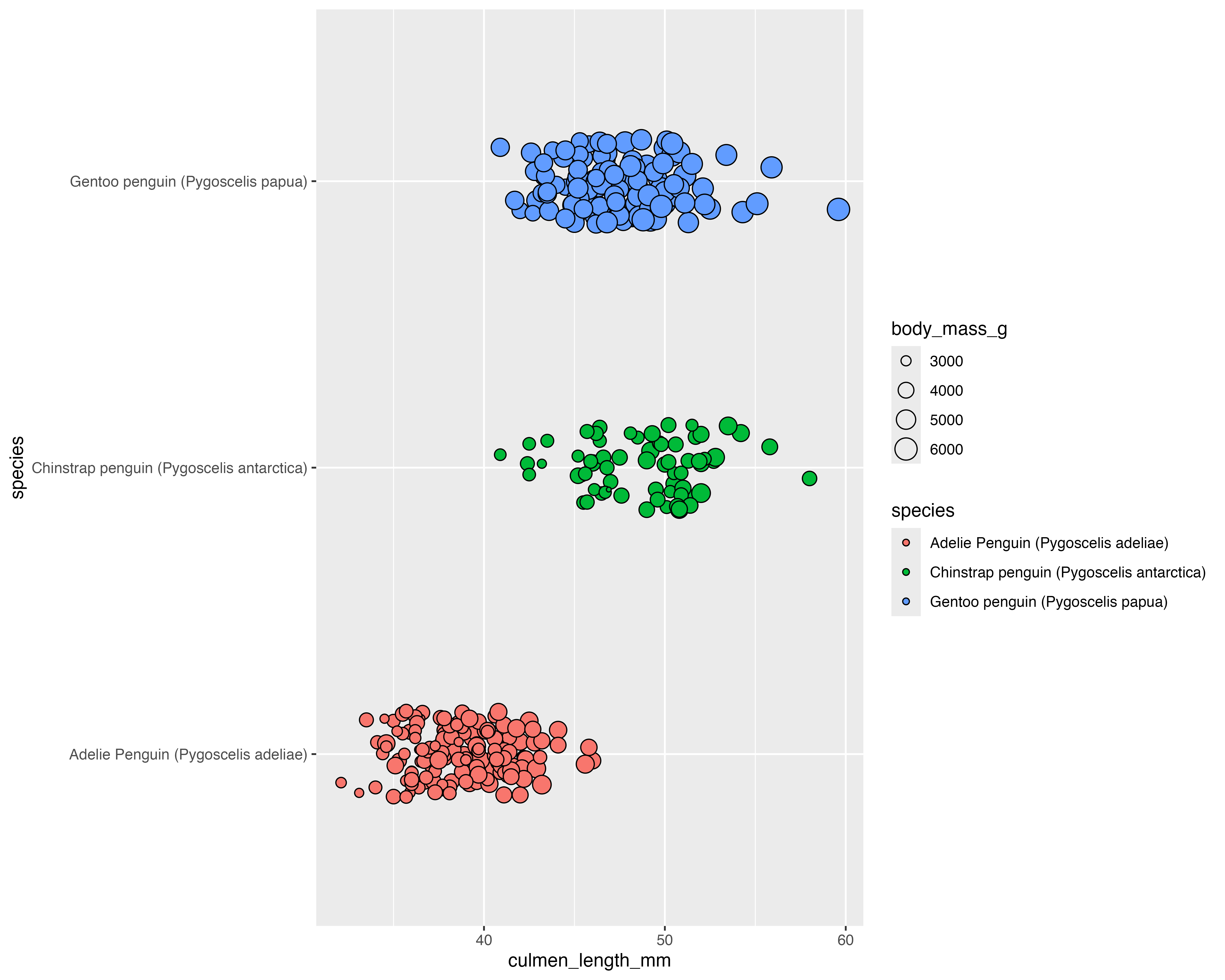
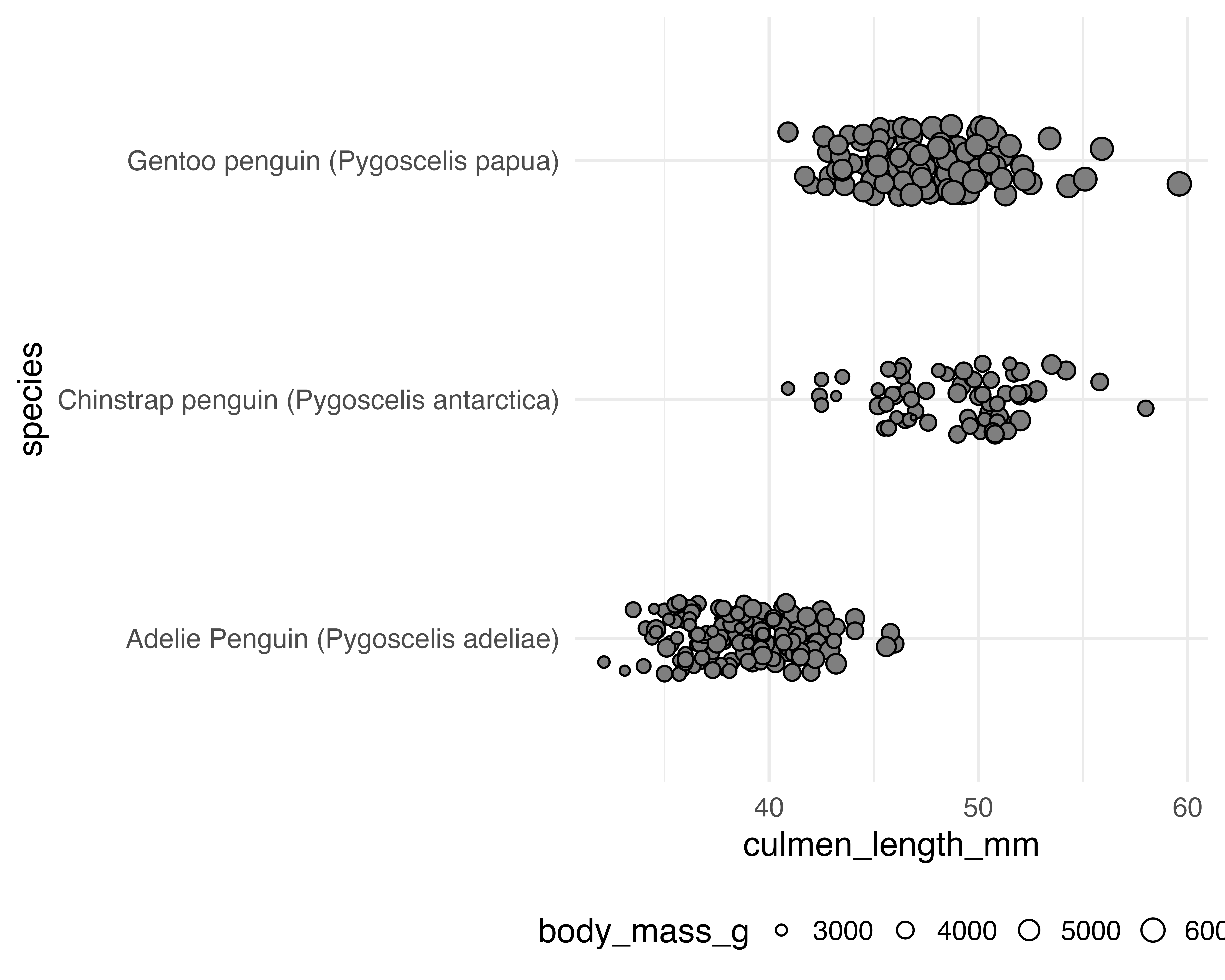
Our starting point
Let’s make a better graph!
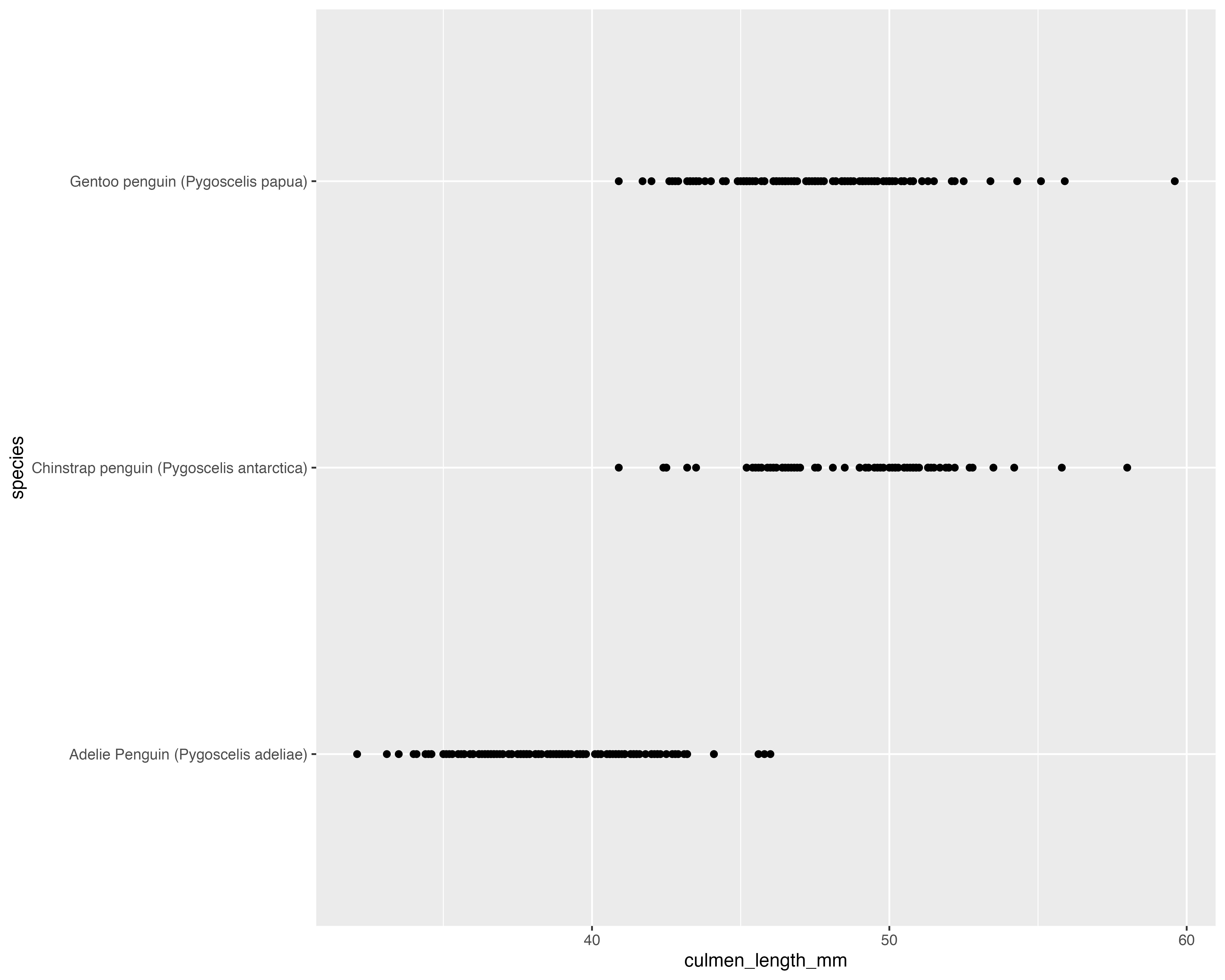
Our starting point
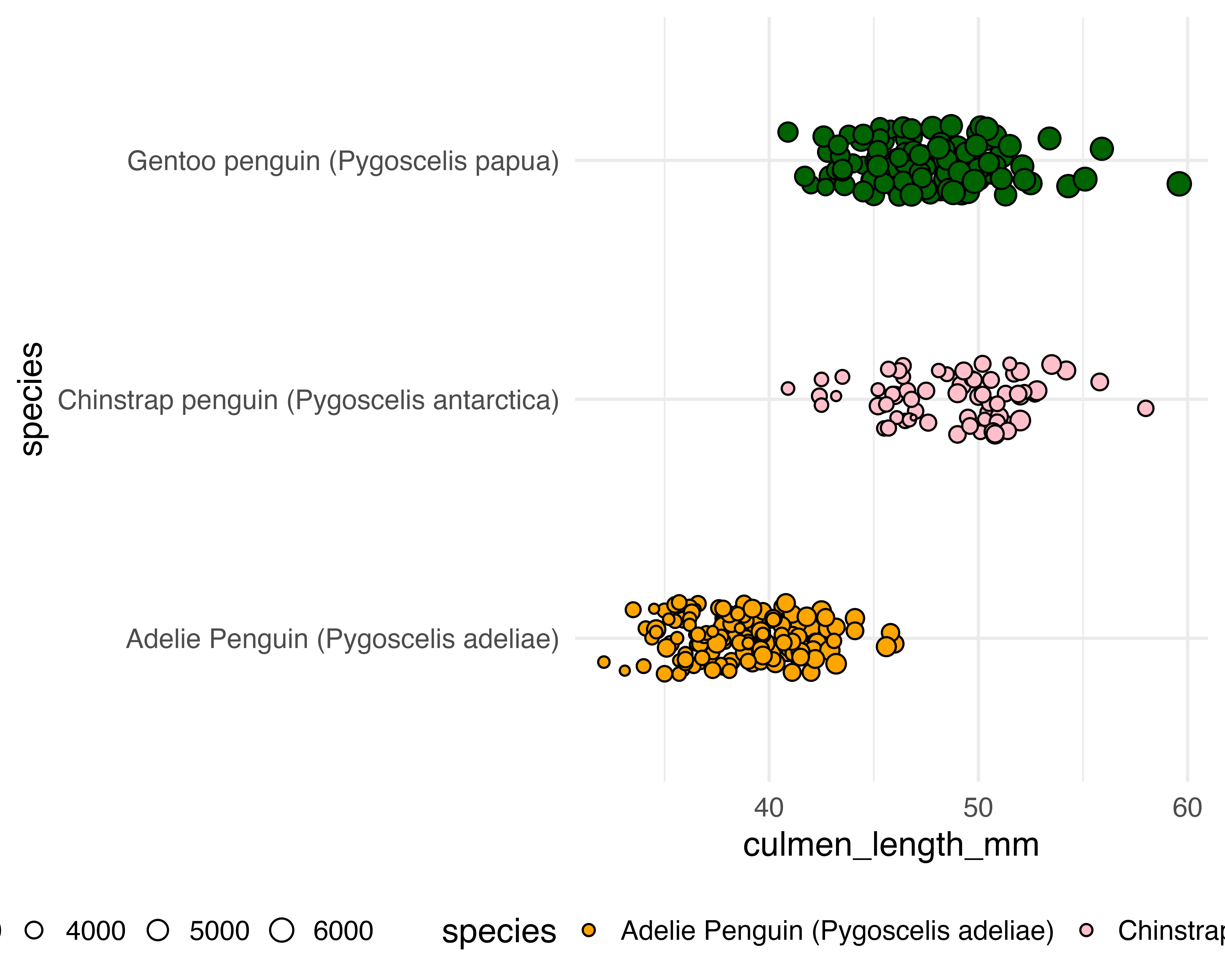
Avoid all the overlaps
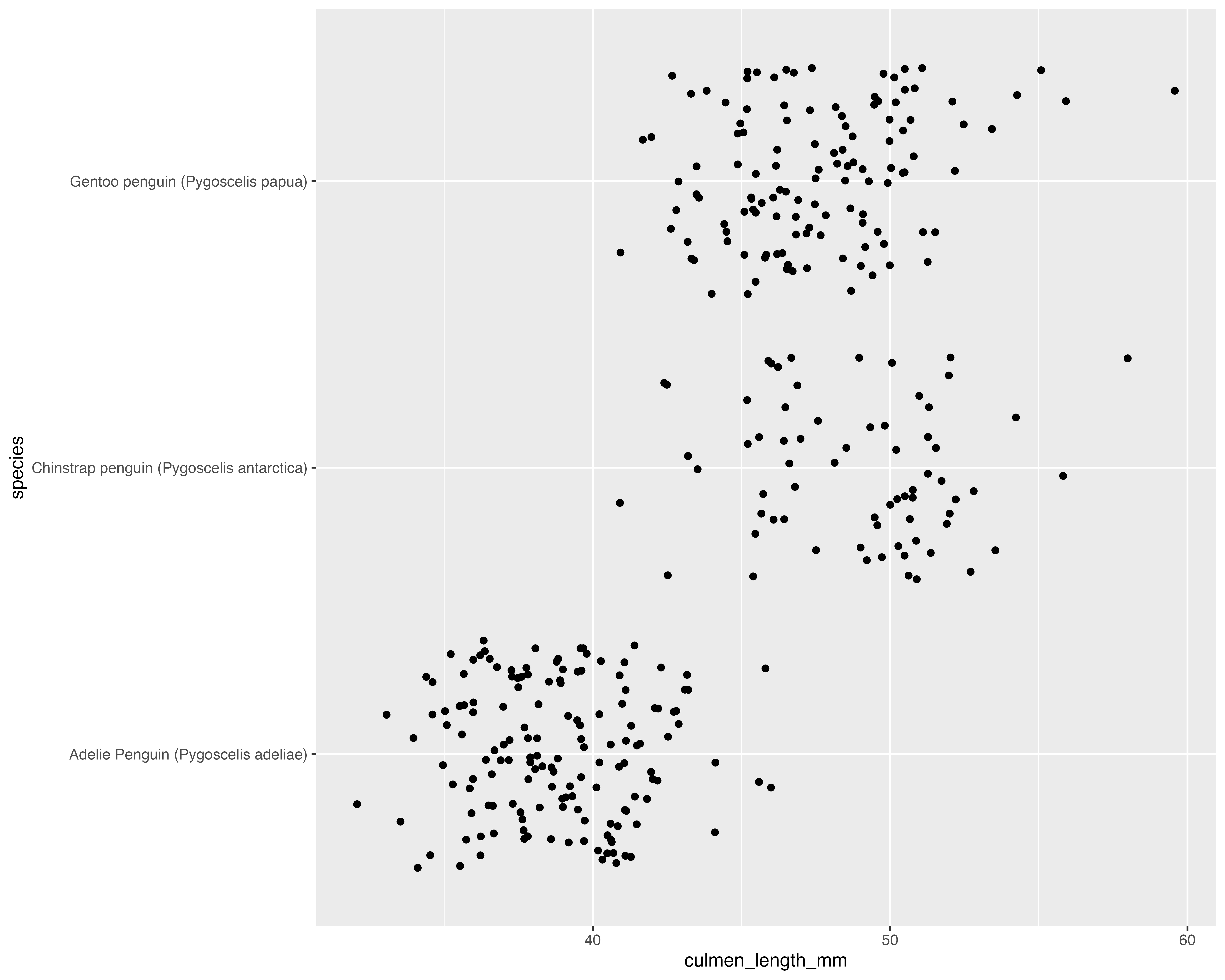
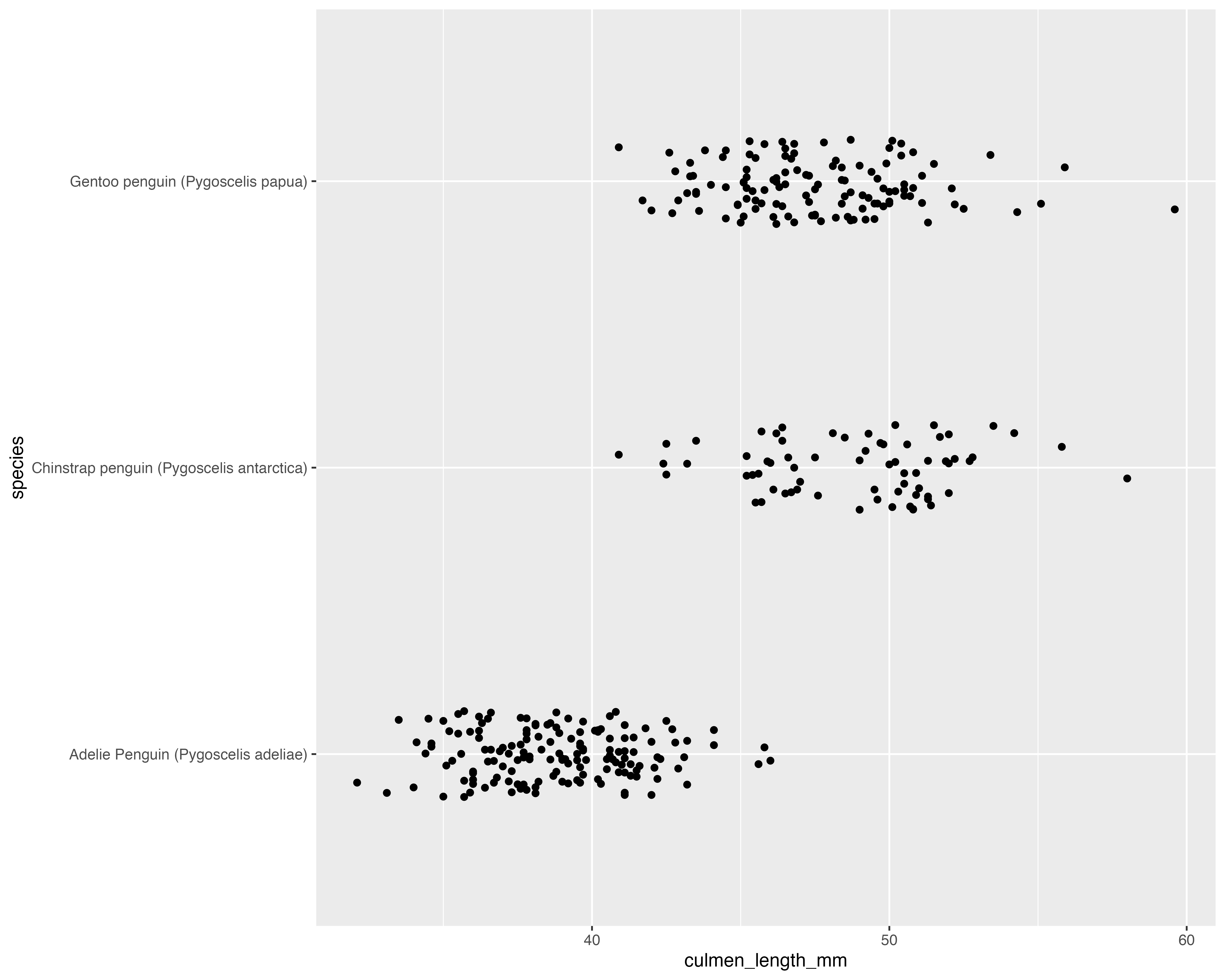
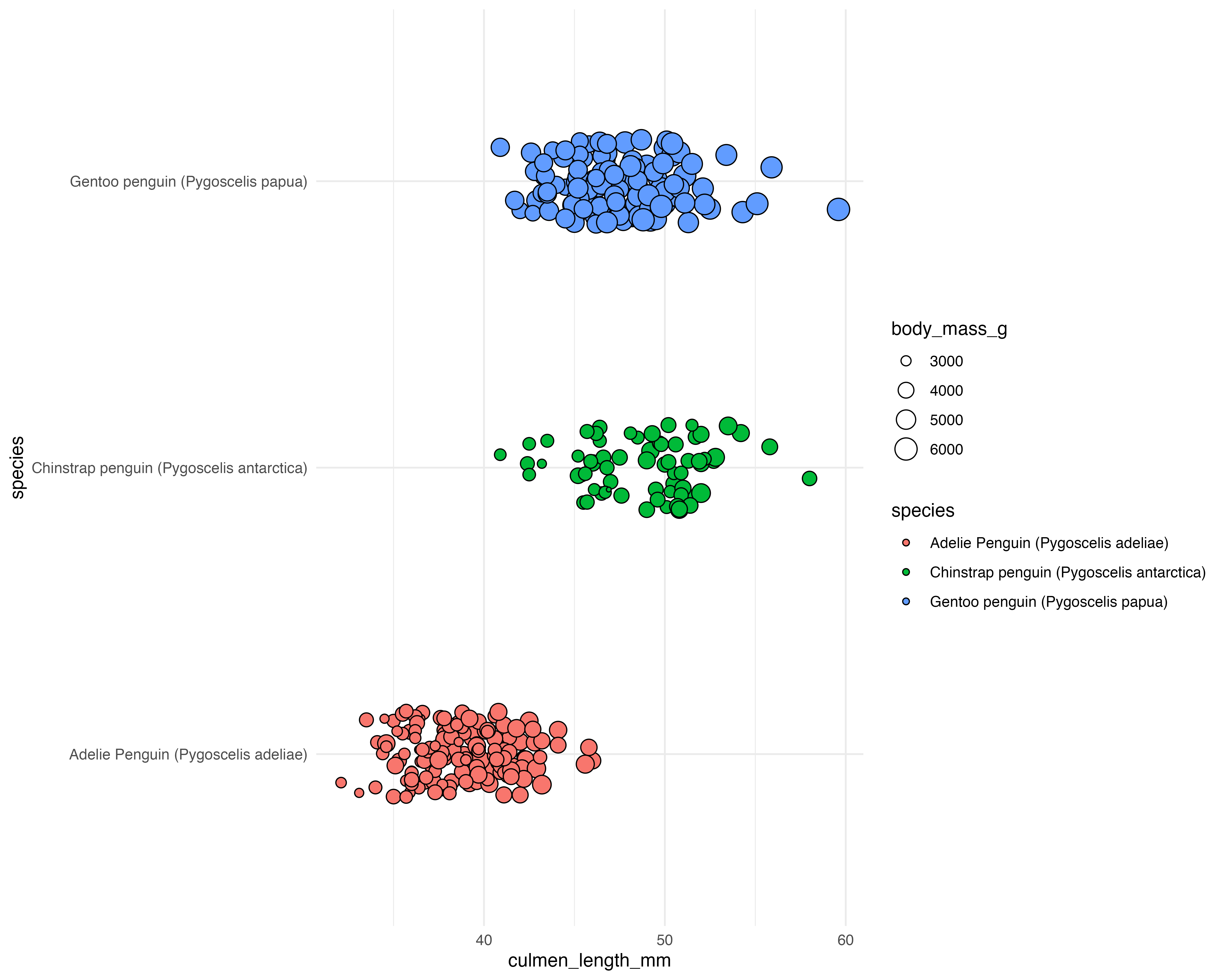
Our starting point
Make the grouping clear, and only jitter what doesn’t matter!
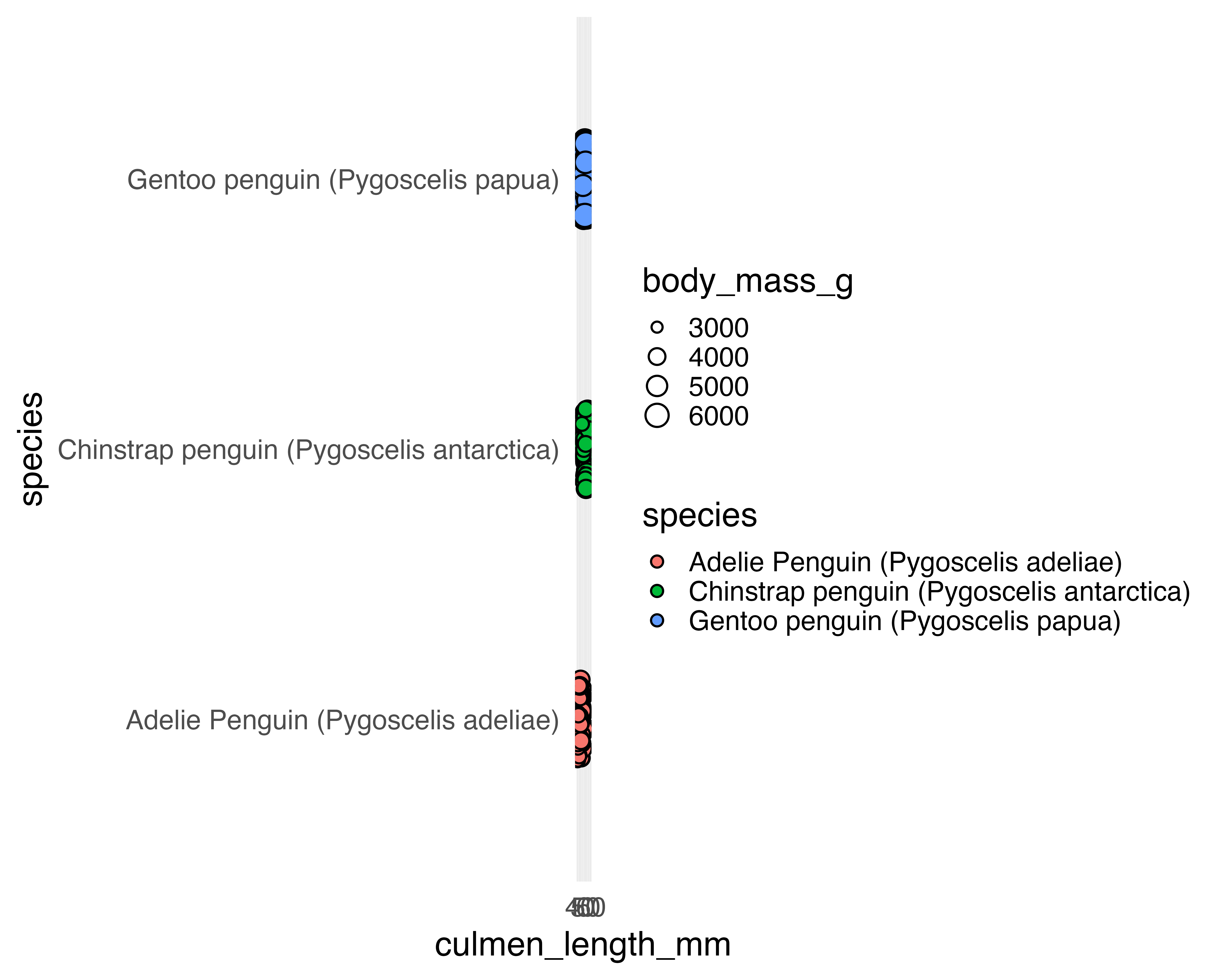
Our starting point
Add a few layers of meaning…
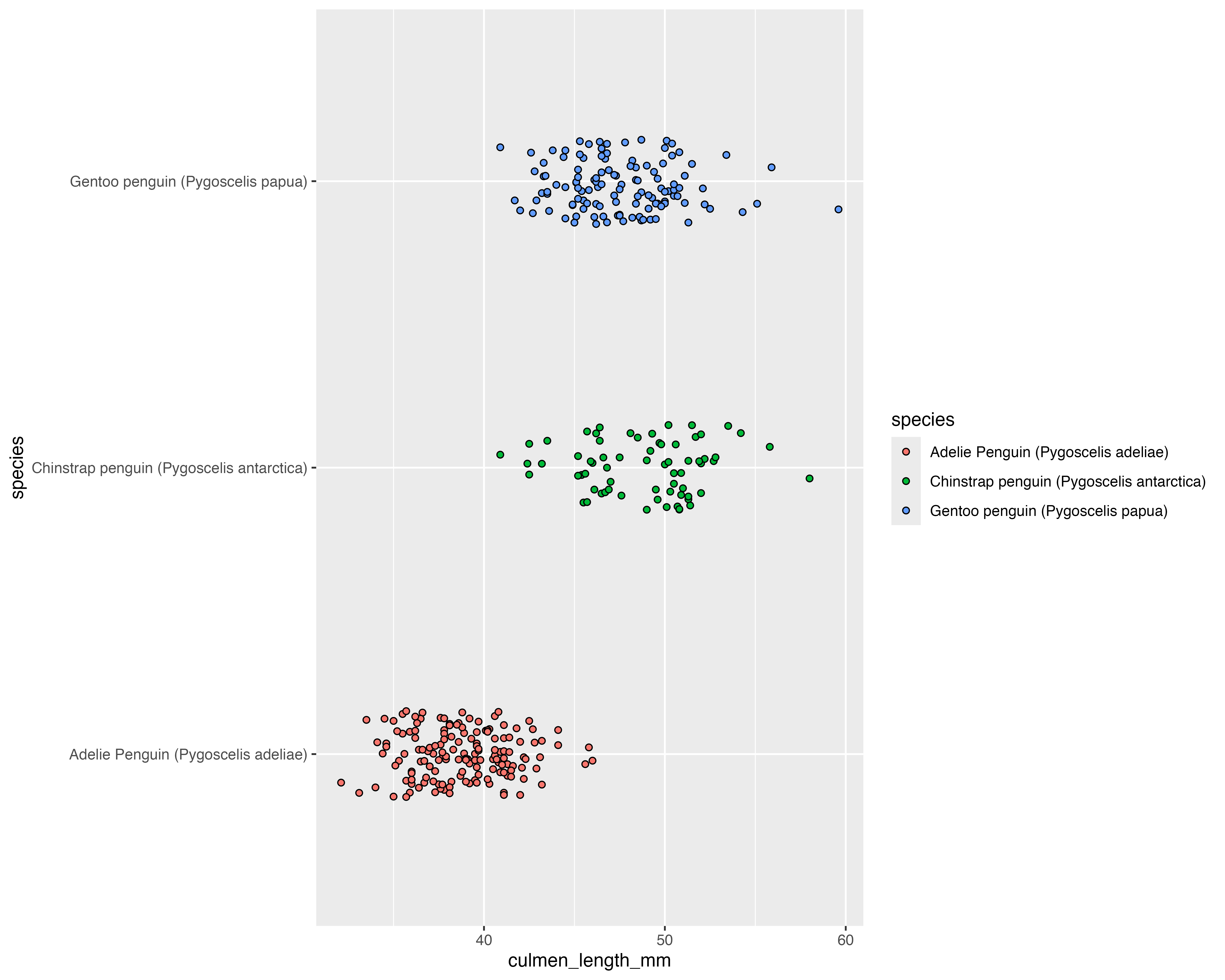
Our starting point
Add a few layers of meaning…
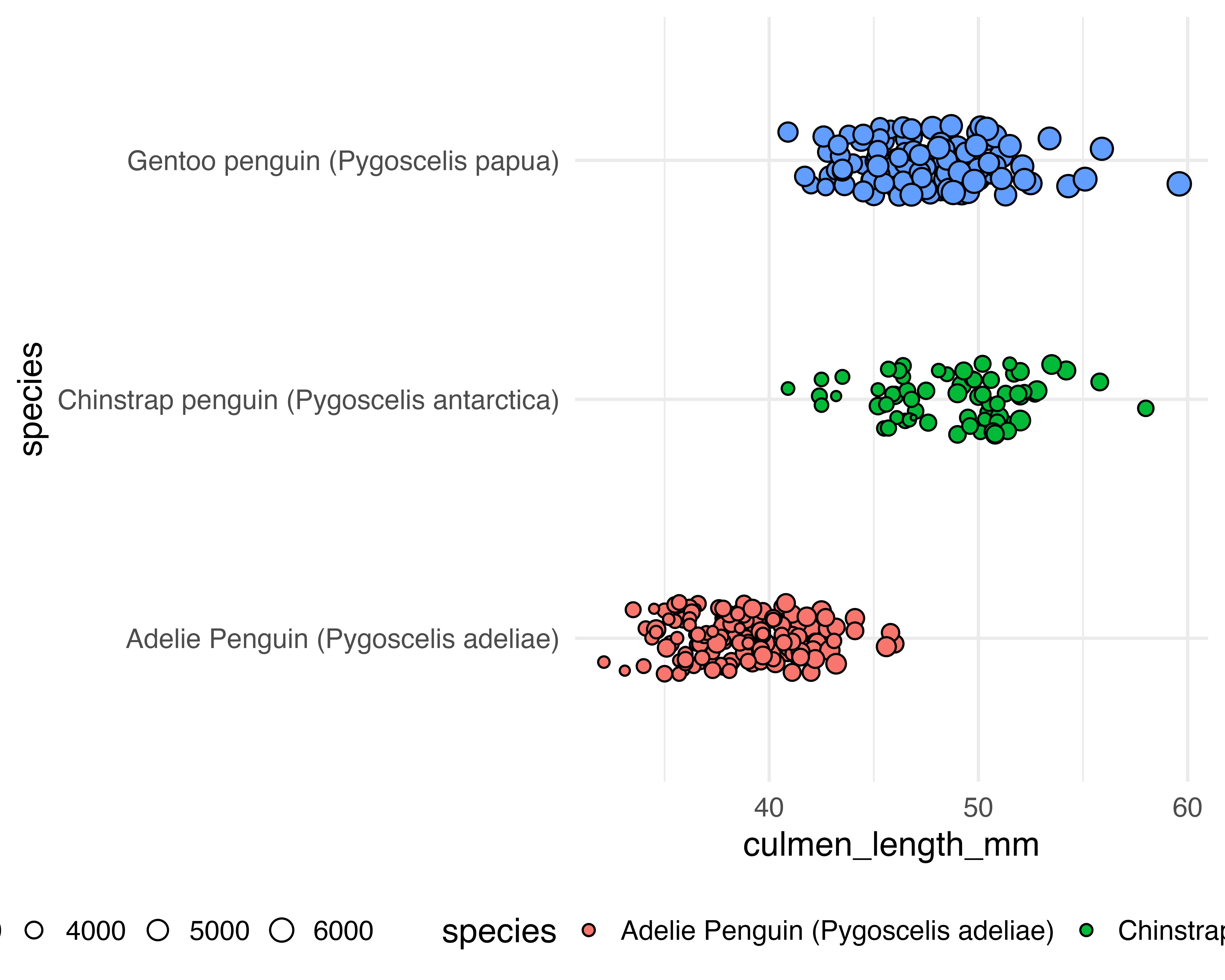
Our starting point
theme_minimal()
Our starting point
theme_minimal()
Our starting point
Move the legend
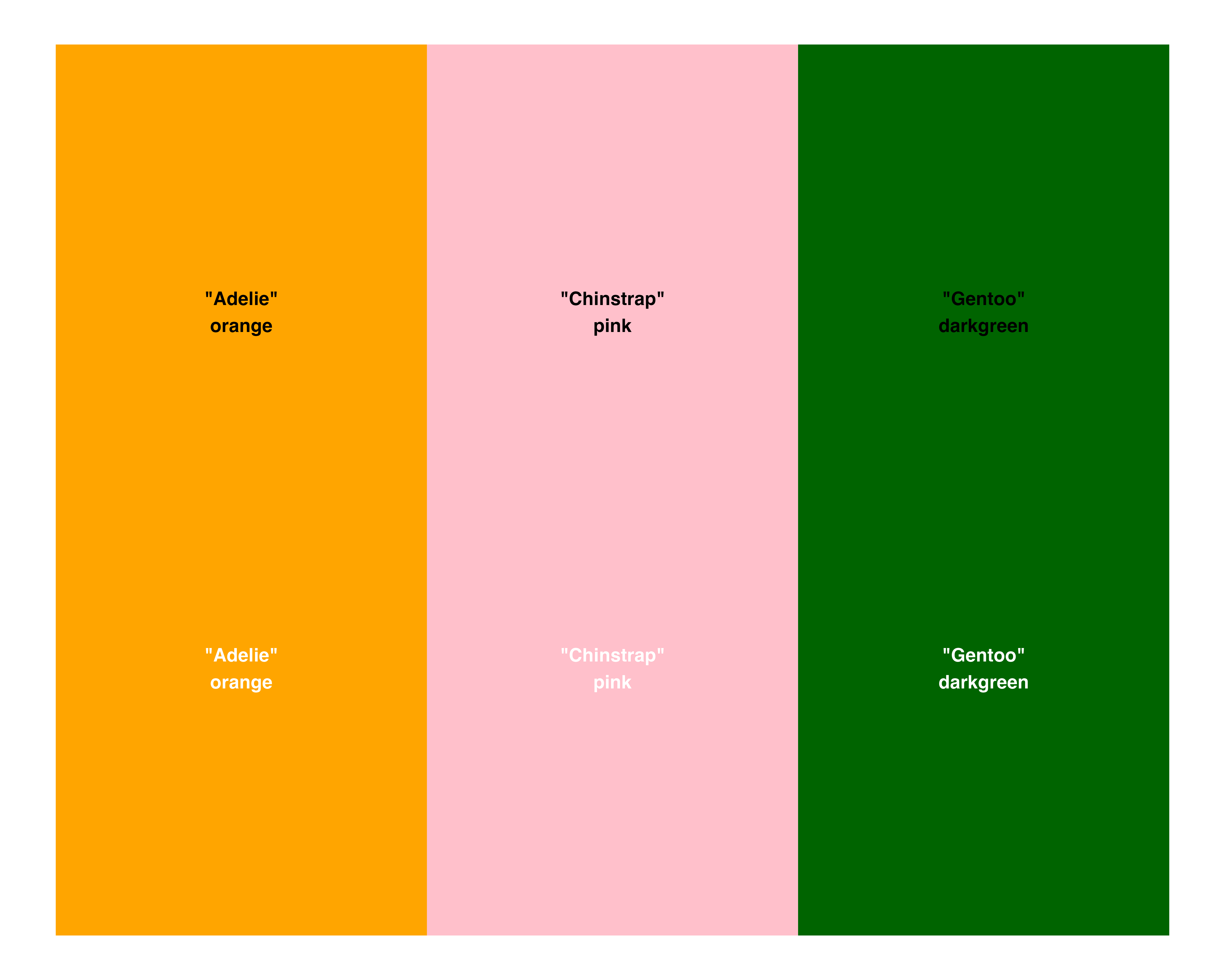
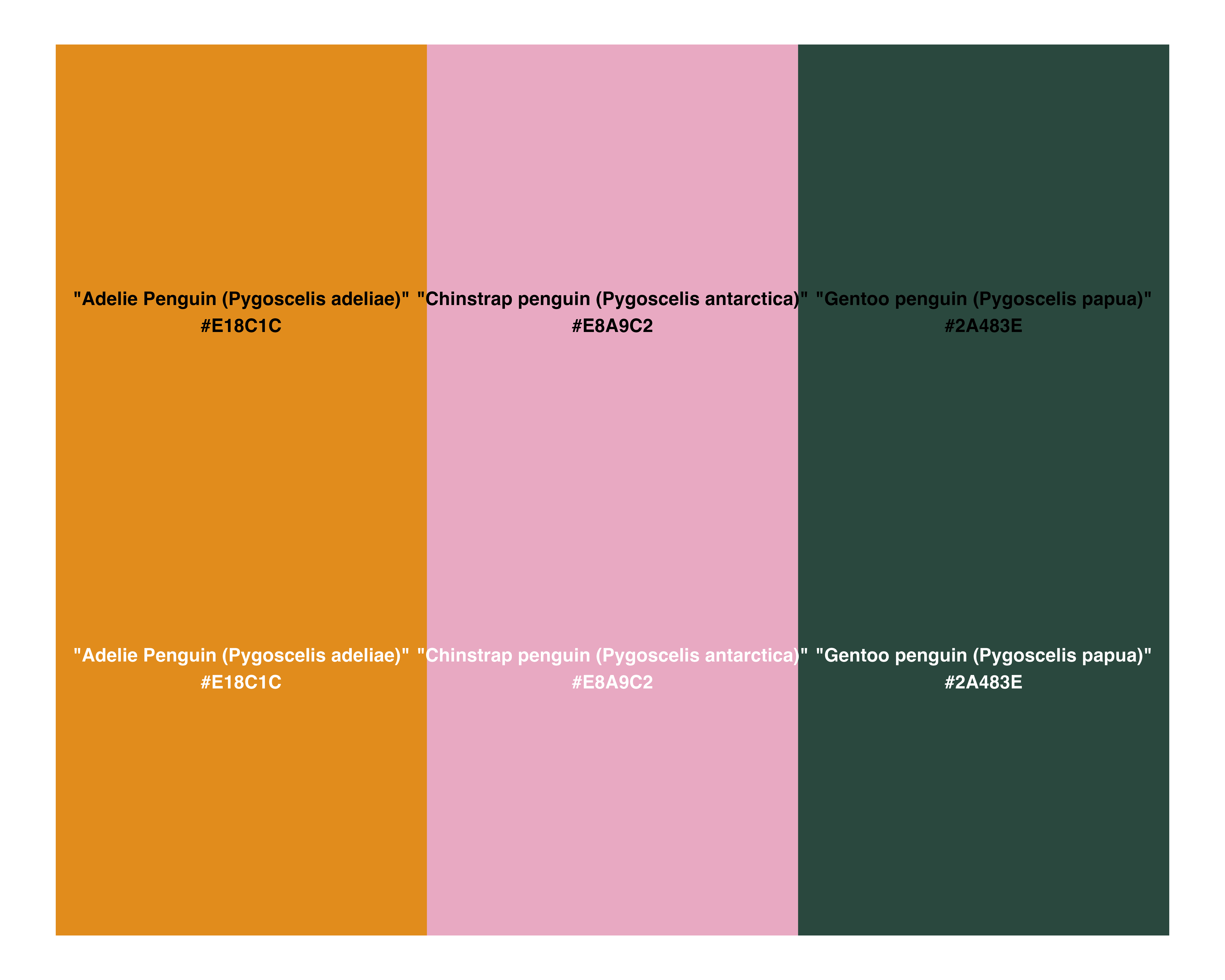
Better colours
- Accessible
- Semantically relevant
- Um…
Starting with the same letter(ish)

Better colours
Blending in a common colour
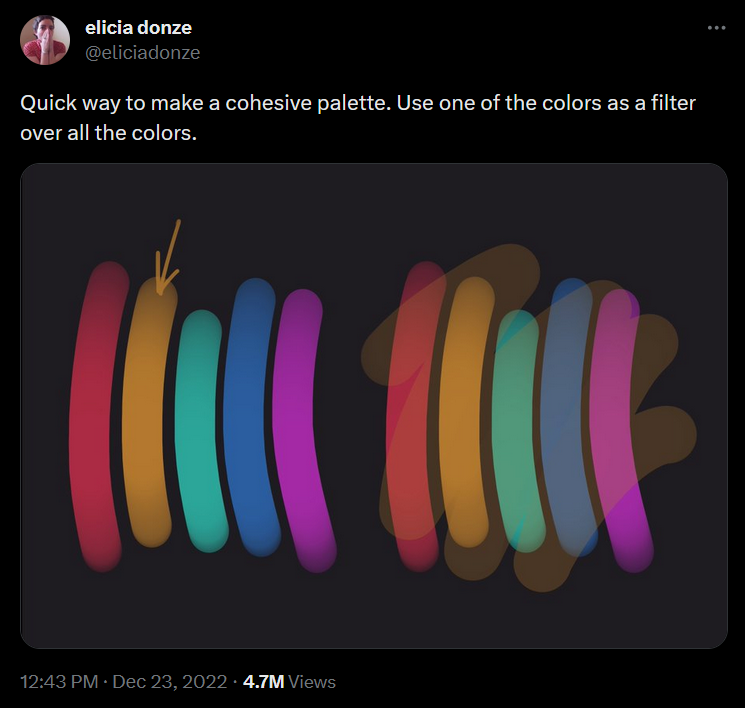
Better colours
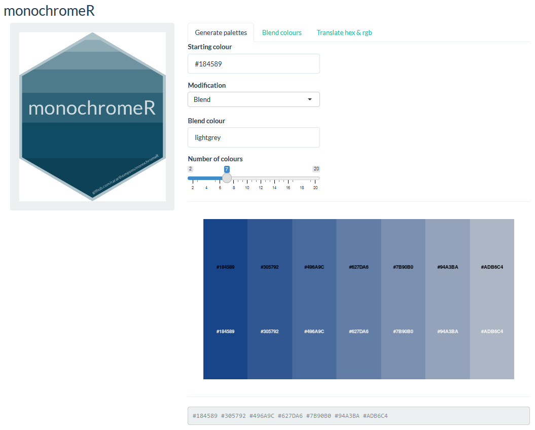
Blending in a common colour - {monochromeR}
🔍 - #6b2c91

Better colours
Blending in a common colour - {monochromeR}
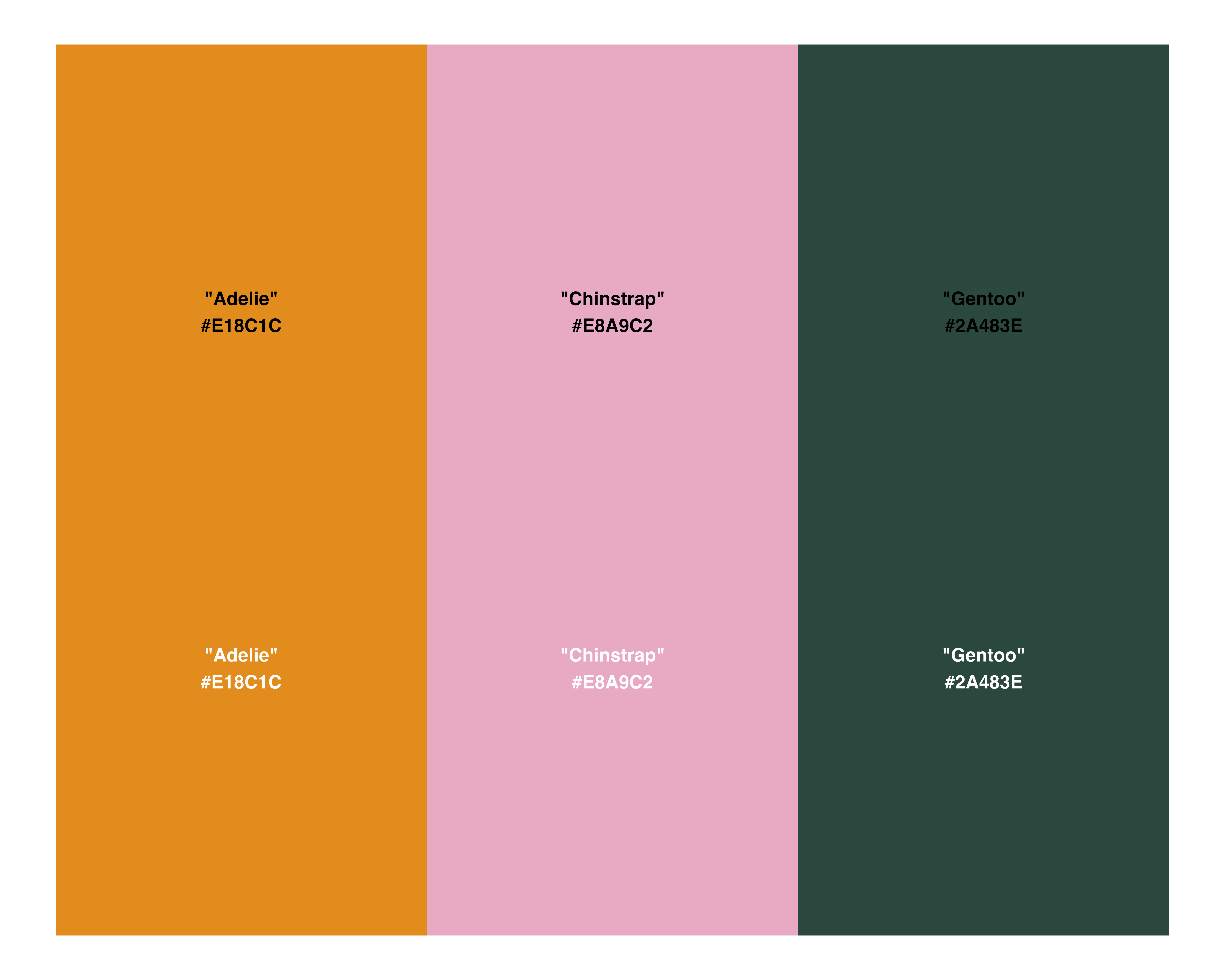
Better colours
It’s subtle… Wait for it!
Better colours
It’s subtle… Wait for it!
Oops!
Named vector needs to match the data!
Better colours
It’s subtle… Wait for it!
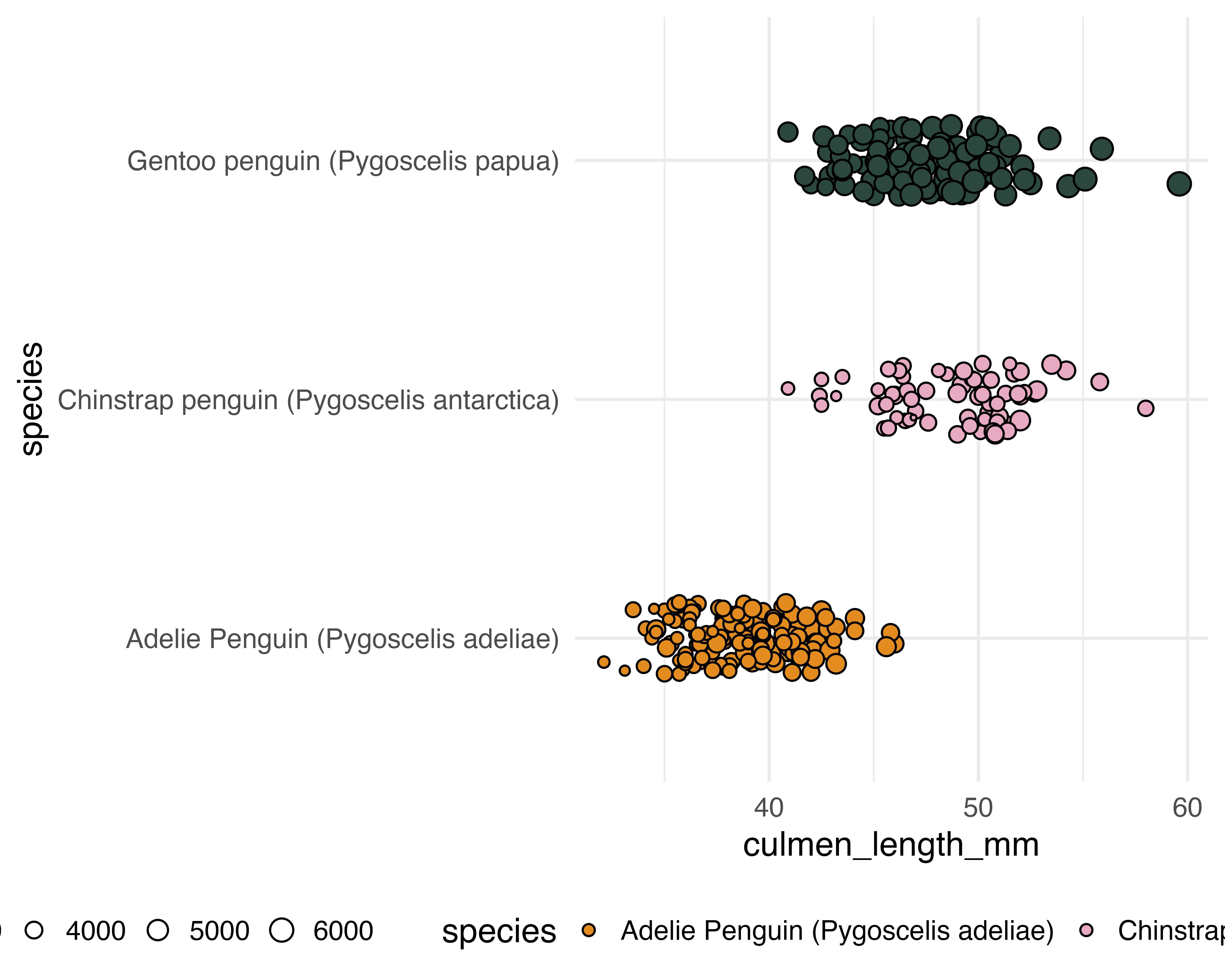
Better colours
It’s subtle… One last thing for now
penguin_df |>
  ggplot() +
  geom_jitter(
    aes(
      x = culmen_length_mm,
      y = species,
      fill = species,
      size = body_mass_g
    ),
    shape = 21,
    width = 0,
    height = 0.15,
    colour = "#333333",
    stroke = 0.5
  ) +
  scale_fill_manual(values = penguin_colours) +
  theme_minimal(base_size = 20) +
  theme(legend.position = "bottom")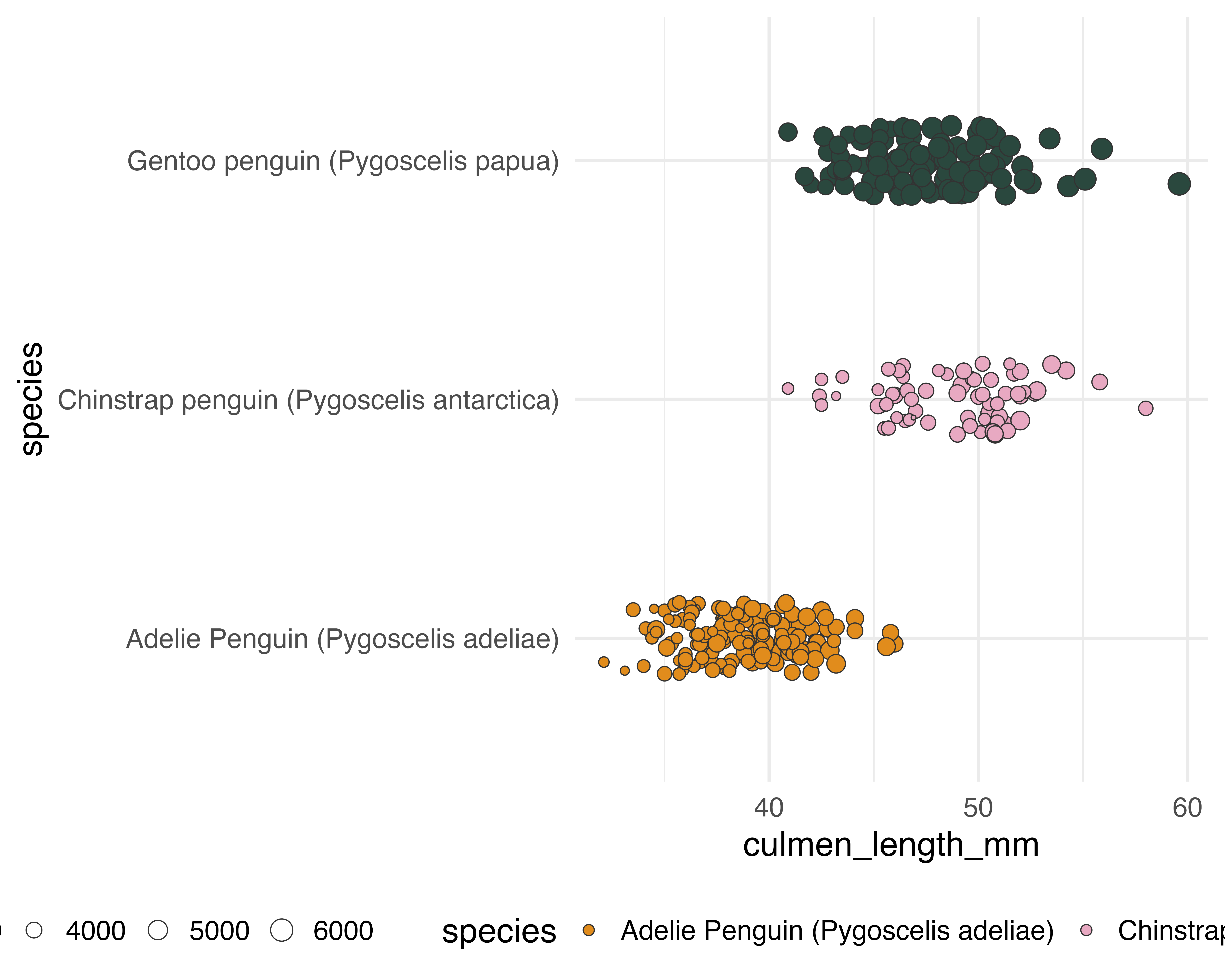
Better text
Did we need the legend? (maybe later?)
penguin_df |>
  ggplot() +
  geom_jitter(
    aes(
      x = culmen_length_mm,
      y = species,
      fill = species,
      size = body_mass_g
    ),
    shape = 21,
    width = 0,
    height = 0.15,
    colour = "#333333",
    stroke = 0.5
  ) +
  scale_fill_manual(values = penguin_colours) +
  theme_minimal(base_size = 20) +
  theme(legend.position = "none")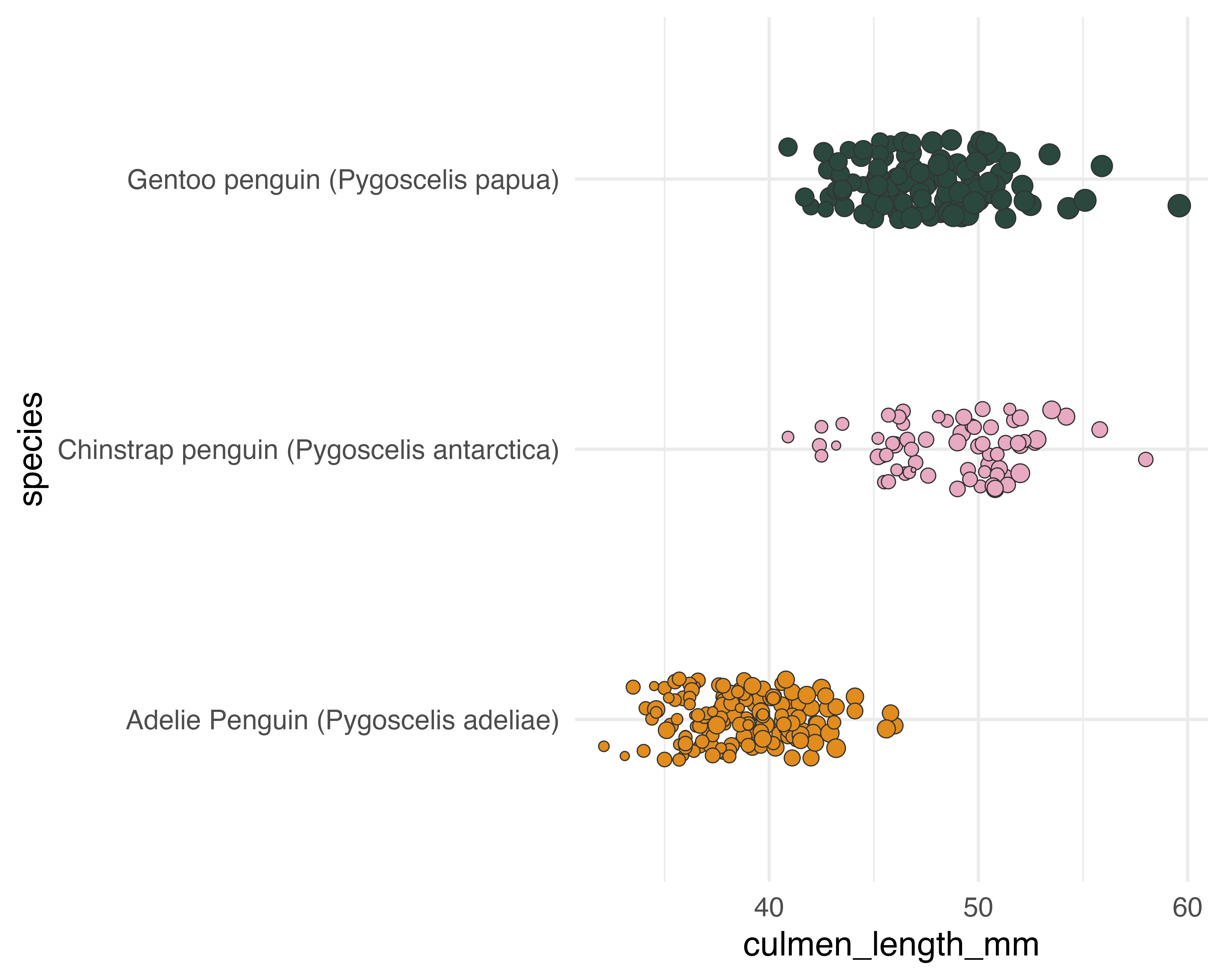
Better text
Or the axis titles?
penguin_df |>
  ggplot() +
  geom_jitter(
    aes(
      x = culmen_length_mm,
      y = species,
      fill = species,
      size = body_mass_g
    ),
    shape = 21,
    width = 0,
    height = 0.15,
    colour = "#333333",
    stroke = 0.5
  ) +
  scale_fill_manual(values = penguin_colours) +
  theme_minimal(base_size = 20) +
  theme(legend.position = "none", axis.title = element_blank())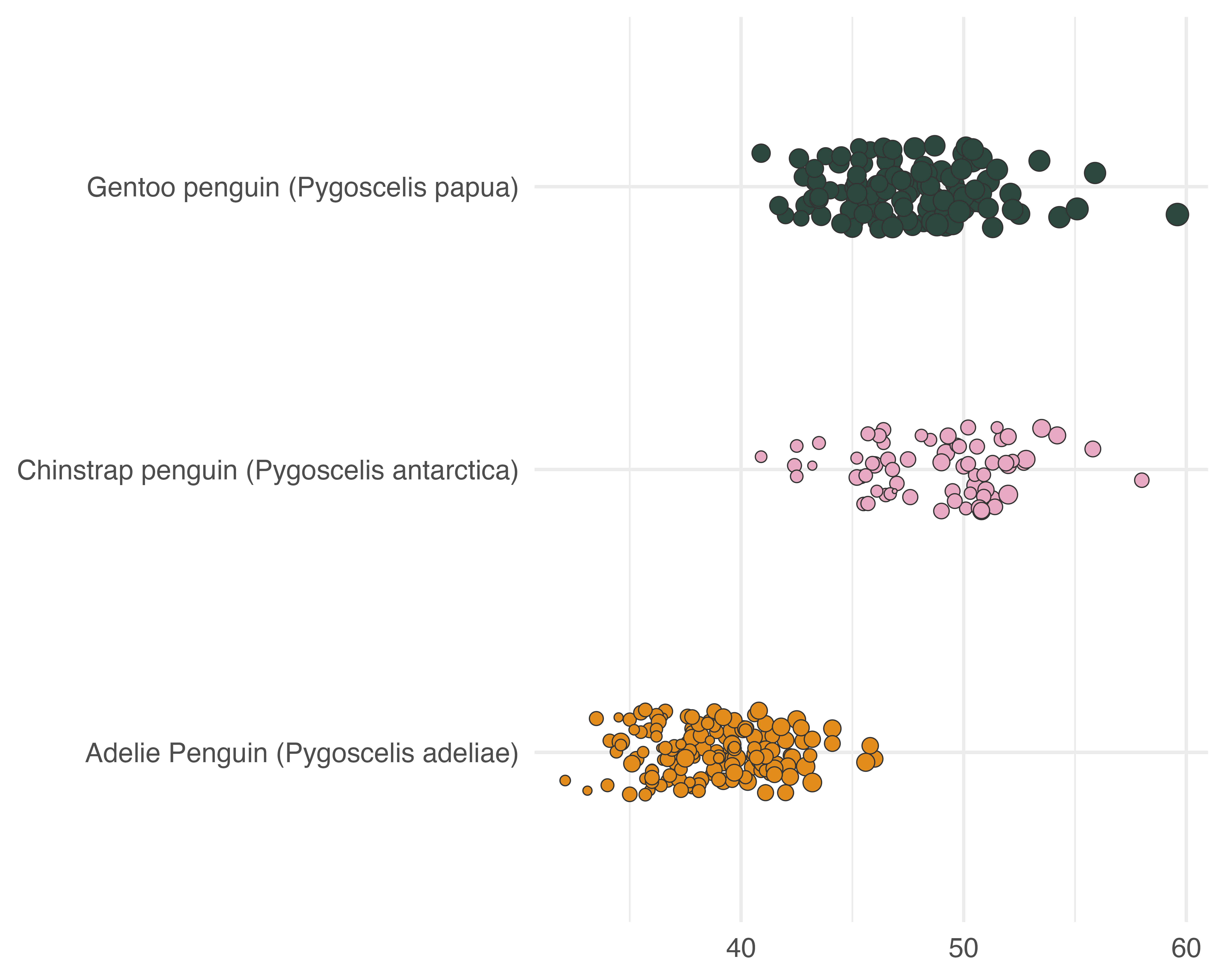
Better text
What about a title?
penguin_df |>
  ggplot() +
  geom_jitter(
    aes(
      x = culmen_length_mm,
      y = species,
      fill = species,
      size = body_mass_g
    ),
    shape = 21,
    width = 0,
    height = 0.15,
    colour = "#333333",
    stroke = 0.5
  ) +
  labs(title = "Beak lengths by species") +
  scale_fill_manual(values = penguin_colours) +
  theme_minimal(base_size = 20) +
  theme(legend.position = "none", axis.title = element_blank())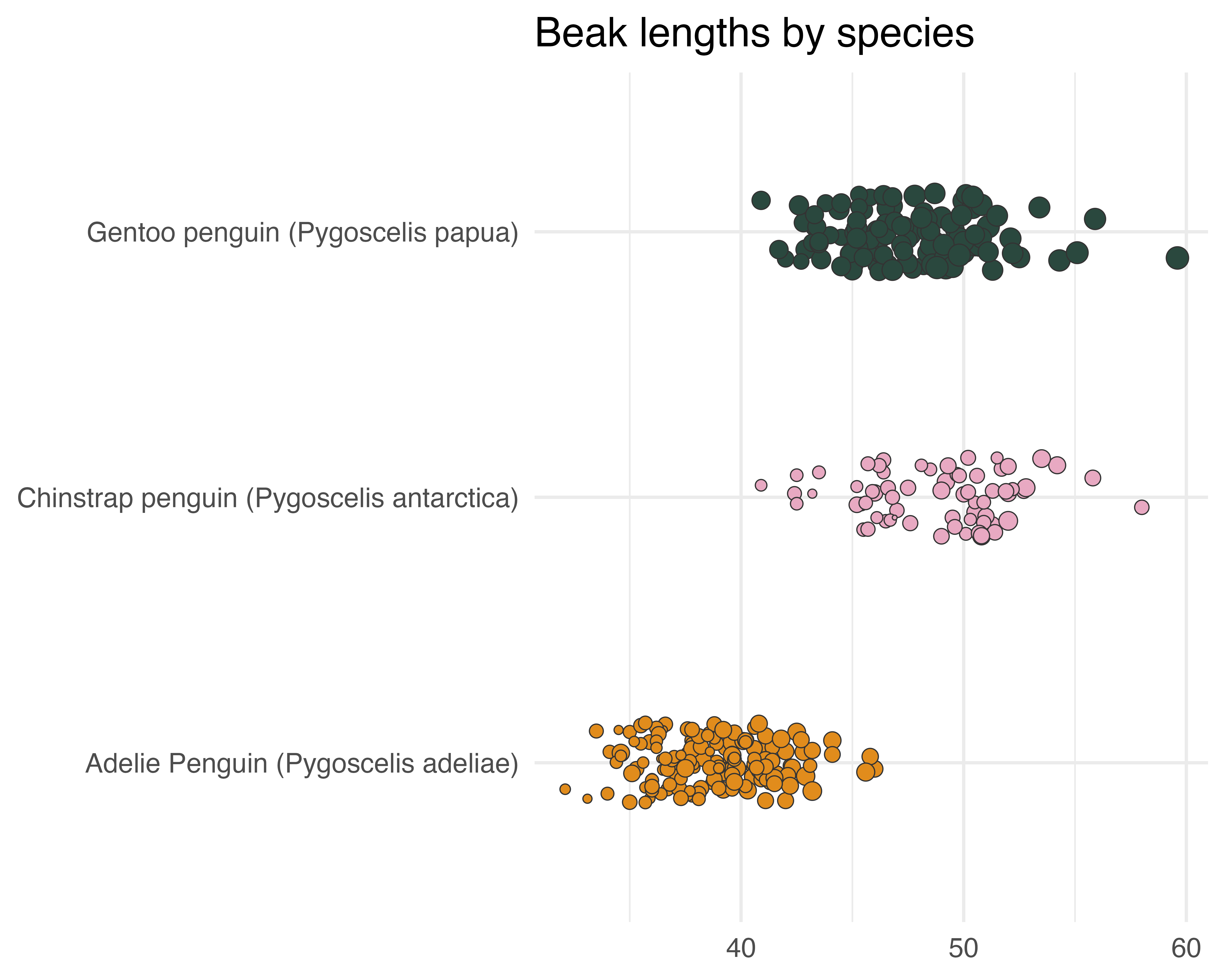
Better text
Let’s be helpful
penguin_df |>
  ggplot() +
  geom_jitter(
    aes(
      x = culmen_length_mm,
      y = species,
      fill = species,
      size = body_mass_g
    ),
    shape = 21,
    width = 0,
    height = 0.15,
    colour = "#333333",
    stroke = 0.5
  ) +
  labs(title = "Beak lengths by species") +
  scale_fill_manual(values = penguin_colours) +
  scale_x_continuous(label = function(x) paste0(x, "mm")) +
  theme_minimal(base_size = 20) +
  theme(legend.position = "none", axis.title = element_blank())
Better text
Sort out the y axis text
penguin_df |>
  ggplot() +
  geom_jitter(
    aes(
      x = culmen_length_mm,
      y = species,
      fill = species,
      size = body_mass_g
    ),
    shape = 21,
    width = 0,
    height = 0.15,
    colour = "#333333",
    stroke = 0.5
  ) +
  labs(title = "Beak lengths by species") +
  scale_fill_manual(values = penguin_colours) +
  scale_x_continuous(label = function(x) paste0(x, "mm")) +
  scale_y_discrete(labels = function(x) gsub("(.)( )(.*)", "\\1", x)) +
  theme_minimal(base_size = 20) +
  theme(legend.position = "none", axis.title = element_blank())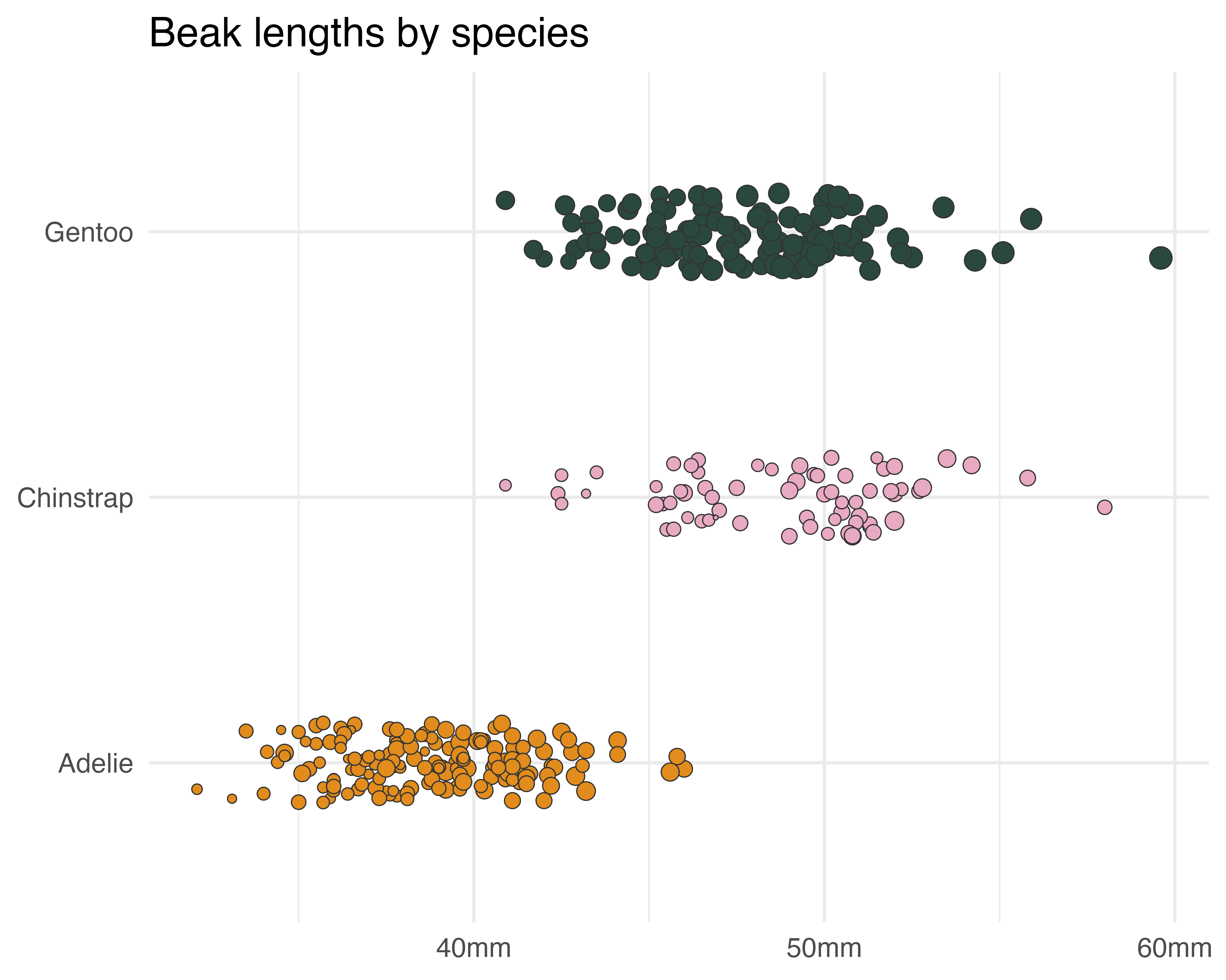
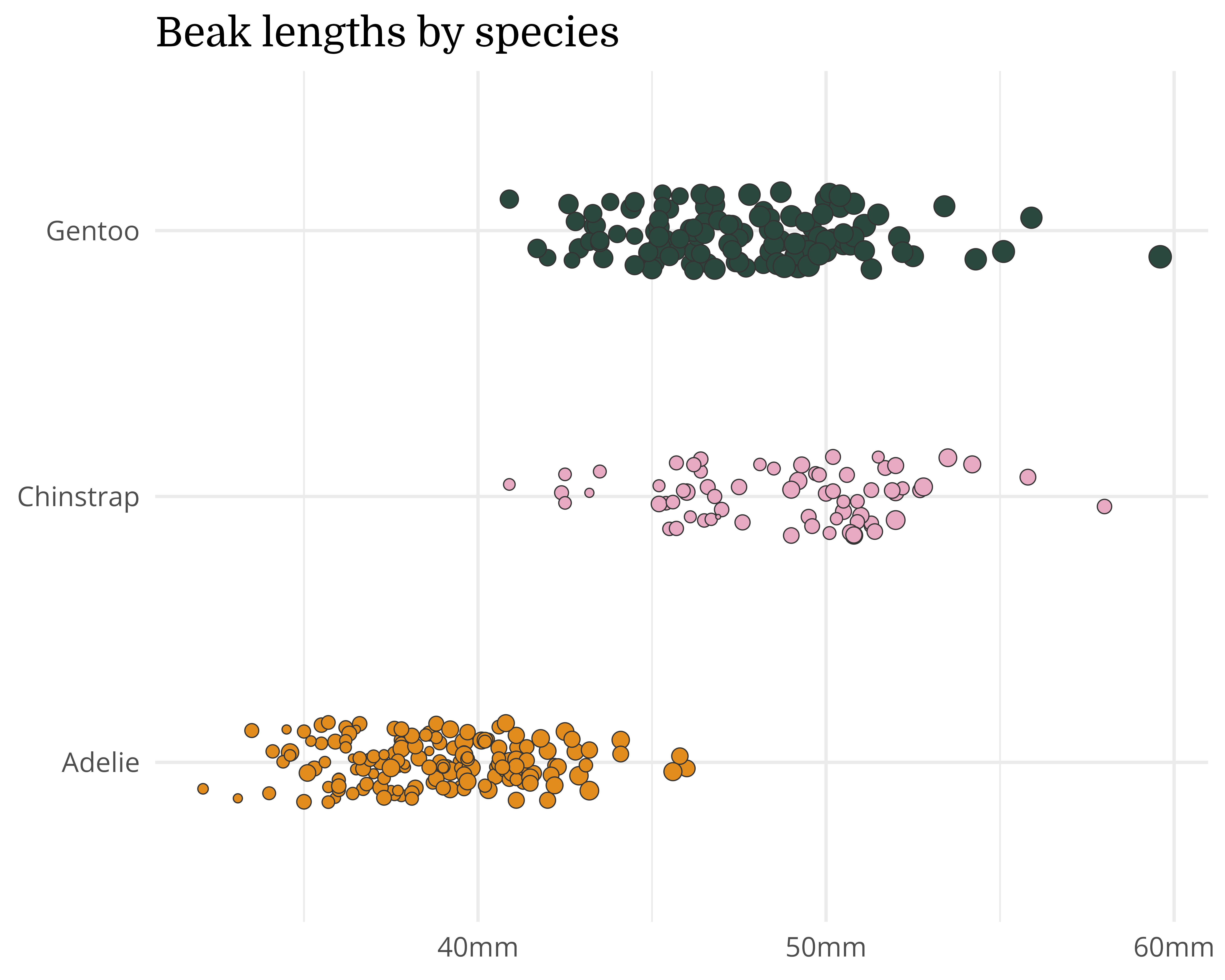
Better text
Better text
Personality
penguin_df |>
  ggplot() +
  geom_jitter(
    aes(
      x = culmen_length_mm,
      y = species,
      fill = species,
      size = body_mass_g
    ),
    shape = 21,
    width = 0,
    height = 0.15,
    colour = "#333333",
    stroke = 0.5
  ) +
  labs(title = "Beak lengths by species") +
  scale_fill_manual(values = penguin_colours) +
  scale_x_continuous(label = function(x) paste0(x, "mm")) +
  scale_y_discrete(labels = function(x) gsub("(.)( )(.*)", "\\1", x)) +
  theme_minimal(base_size = 20) +
  theme(
    text = element_text(family = "Open Sans"),
    legend.position = "none",
    axis.title = element_blank(),
    plot.title = element_text(family = "Domine")
  )
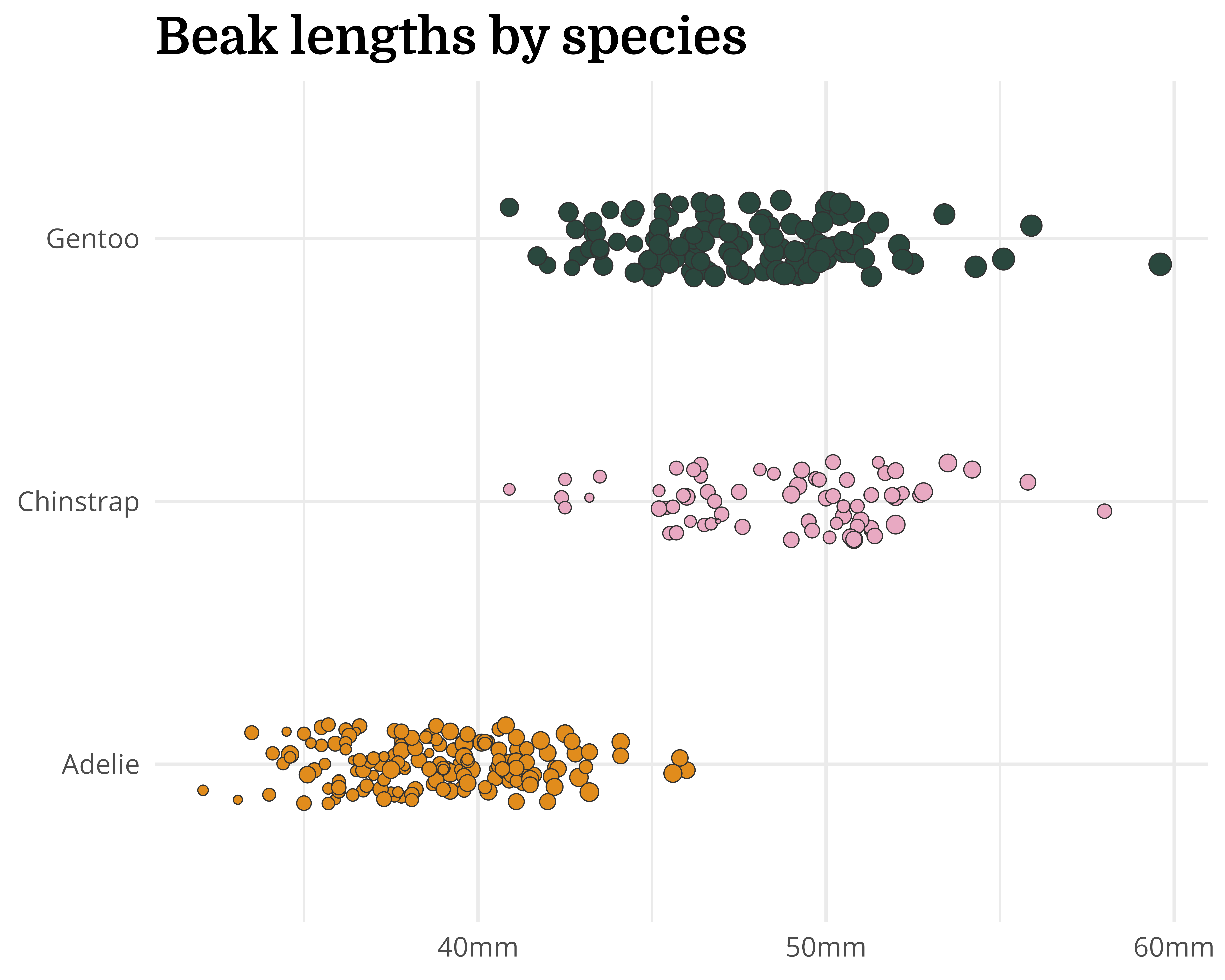
Better text
Personality + hierarchy
penguin_df |>
  ggplot() +
  geom_jitter(
    aes(
      x = culmen_length_mm,
      y = species,
      fill = species,
      size = body_mass_g
    ),
    shape = 21,
    width = 0,
    height = 0.15,
    colour = "#333333",
    stroke = 0.5
  ) +
  labs(title = "Beak lengths by species") +
  scale_fill_manual(values = penguin_colours) +
  scale_x_continuous(label = function(x) paste0(x, "mm")) +
  scale_y_discrete(labels = function(x) gsub("(.)( )(.*)", "\\1", x)) +
  theme_minimal(base_size = 20) +
  theme(
    text = element_text(family = "Open Sans"),
    legend.position = "none",
    axis.title = element_blank(),
    plot.title = element_text(
      family = "Domine",
      face = "bold",
      size = 30
    )
  )
Better text
Personality + hierarchy (better!)
penguin_df |>
  ggplot() +
  geom_jitter(
    aes(
      x = culmen_length_mm,
      y = species,
      fill = species,
      size = body_mass_g
    ),
    shape = 21,
    width = 0,
    height = 0.15,
    colour = "#333333",
    stroke = 0.5
  ) +
  labs(title = "Beak lengths by species") +
  scale_fill_manual(values = penguin_colours) +
  scale_x_continuous(label = function(x) paste0(x, "mm")) +
  scale_y_discrete(labels = function(x) gsub("(.)( )(.*)", "\\1", x)) +
  theme_minimal(base_size = 20) +
  theme(
    text = element_text(family = "Open Sans"),
    legend.position = "none",
    axis.title = element_blank(),
    plot.title = element_text(
      family = "Domine",
      face = "bold",
      size = rel(1.5)
    )
  )
Better text
Personality + hierarchy + colour
penguin_df |>
  ggplot() +
  geom_jitter(
    aes(
      x = culmen_length_mm,
      y = species,
      fill = species,
      size = body_mass_g
    ),
    shape = 21,
    width = 0,
    height = 0.15,
    colour = "#333333",
    stroke = 0.5
  ) +
  labs(title = "Beak lengths by species") +
  scale_fill_manual(values = penguin_colours) +
  scale_x_continuous(label = function(x) paste0(x, "mm")) +
  scale_y_discrete(labels = function(x) gsub("(.)( )(.*)", "\\1", x)) +
  theme_minimal(base_size = 20) +
  theme(
    text = element_text(family = "Open Sans", colour = "#534959"),
    axis.text = element_text(colour = "#534959"),
    legend.position = "none",
    axis.title = element_blank(),
    plot.title = element_text(
      family = "Domine",
      face = "bold",
      size = rel(1.5),
      colour = "#15081D"
    )
  )
Getting fonts to work in R
Getting fonts to work can be frustrating!
Install fonts locally, restart R Studio + 📦
{systemfonts}({ragg}+{textshaping}) + Set graphics device to “AGG” + 🤞
knitr::opts_chunk$set(dev = “ragg_png”)
Optimise the small things
Background, grid, margins…
penguin_df |>
  ggplot() +
  geom_jitter(
    aes(
      x = culmen_length_mm,
      y = species,
      fill = species,
      size = body_mass_g
    ),
    shape = 21,
    width = 0,
    height = 0.15,
    colour = "#333333",
    stroke = 0.5
  ) +
  labs(title = "Beak lengths by species") +
  scale_fill_manual(values = penguin_colours) +
  scale_x_continuous(label = function(x) paste0(x, "mm")) +
  scale_y_discrete(labels = function(x) gsub("(.)( )(.*)", "\\1", x)) +
  theme_minimal(base_size = 20) +
  theme(
    text = element_text(family = "Open Sans", colour = "#534959"),
    axis.text = element_text(colour = "#534959"),
    legend.position = "none",
    axis.title = element_blank(),
    plot.title.position = "plot",
    plot.title = element_text(
      family = "Domine",
      face = "bold",
      size = rel(1.5),
      colour = "#15081D",
      margin = margin(0, 0, 20, 0)
    ),
    panel.grid = element_line(colour = "#FFFFFF"),
    plot.background = element_rect(fill = "#f9f5fc", colour = "#f9f5fc"),
    plot.margin = margin_auto(30)
  )
Helping your future self
Plot
Helping your future self
Plot + theme_chester_penguins()
Helping your future self
Plot
Helping your future self
Plots + theme_chester_penguins() (or theme_{your-research-group}()?)
Shameless plug alert!
Plots + theme_{your-research-group}()?
Shameless plug alert!
Plots + theme_{your-research-group}()?
Shameless plug alert!
Plots + theme_{your-research-group}()?
Annotations
Highlight the overall range…
beak_range_df <- penguin_df |>
  dplyr::filter(
    culmen_length_mm == max(culmen_length_mm, na.rm = TRUE) |
      culmen_length_mm == min(culmen_length_mm, na.rm = TRUE)
  )

penguin_df |>
  ggplot() +
  geom_jitter(
    aes(
      x = culmen_length_mm,
      y = species,
      fill = species,
      size = body_mass_g
    ),
    shape = 21,
    width = 0,
    height = 0.15,
    colour = "#333333",
    stroke = 0.5
  ) +
  geom_vline(
    data = beak_range_df,
    aes(xintercept = culmen_length_mm),
    linetype = 3
  ) +
  labs(title = "Beak lengths by species") +
  scale_fill_manual(values = penguin_colours) +
  scale_x_continuous(label = function(x) paste0(x, "mm")) +
  scale_y_discrete(labels = function(x) gsub("(.)( )(.*)", "\\1", x)) +
  theme_chester_penguins()
Annotations
Move to background + change colour
penguin_df |>
  ggplot() +
  geom_vline(
    data = beak_range_df,
    aes(xintercept = culmen_length_mm),
    linetype = 3,
    colour = "#333333"
  ) +
  geom_jitter(
    aes(
      x = culmen_length_mm,
      y = species,
      fill = species,
      size = body_mass_g
    ),
    shape = 21,
    width = 0,
    height = 0.15,
    colour = "#333333",
    stroke = 0.5
  ) +
  labs(title = "Beak lengths by species") +
  scale_fill_manual(values = penguin_colours) +
  scale_x_continuous(label = function(x) paste0(x, "mm")) +
  scale_y_discrete(labels = function(x) gsub("(.)( )(.*)", "\\1", x)) +
  theme_chester_penguins()
Annotations
Add labels
penguin_df |>
  ggplot(aes(x = culmen_length_mm, y = species)) +
  geom_vline(
    data = beak_range_df,
    aes(xintercept = culmen_length_mm),
    linetype = 3,
    colour = "#333333"
  ) +
  geom_jitter(
    aes(
      x = culmen_length_mm,
      y = species,
      fill = species,
      size = body_mass_g
    ),
    shape = 21,
    width = 0,
    height = 0.15,
    colour = "#333333",
    stroke = 0.5
  ) +
  ggtext::geom_textbox(
    data = beak_range_df,
    aes(label = paste0(culmen_length_mm, "mm"))
  ) +
  labs(title = "Beak lengths by species") +
  scale_fill_manual(values = penguin_colours) +
  scale_x_continuous(label = function(x) paste0(x, "mm")) +
  scale_y_discrete(labels = function(x) gsub("(.)( )(.*)", "\\1", x)) +
  theme_chester_penguins()
Annotations
Add labels
penguin_df |>
  ggplot(aes(x = culmen_length_mm, y = species)) +
  geom_vline(
    data = beak_range_df,
    aes(xintercept = culmen_length_mm),
    linetype = 3,
    colour = "#333333"
  ) +
  geom_jitter(
    aes(
      x = culmen_length_mm,
      y = species,
      fill = species,
      size = body_mass_g
    ),
    shape = 21,
    width = 0,
    height = 0.15,
    colour = "#333333",
    stroke = 0.5
  ) +
  ggtext::geom_textbox(
    data = beak_range_df,
    aes(label = paste0(culmen_length_mm, "mm")),
    family = "Open Sans",
    halign = 0.5,
    colour = "#333333",
    fill = NA
  ) +
  labs(title = "Beak lengths by species") +
  scale_fill_manual(values = penguin_colours) +
  scale_x_continuous(label = function(x) paste0(x, "mm")) +
  scale_y_discrete(labels = function(x) gsub("(.)( )(.*)", "\\1", x)) +
  theme_chester_penguins()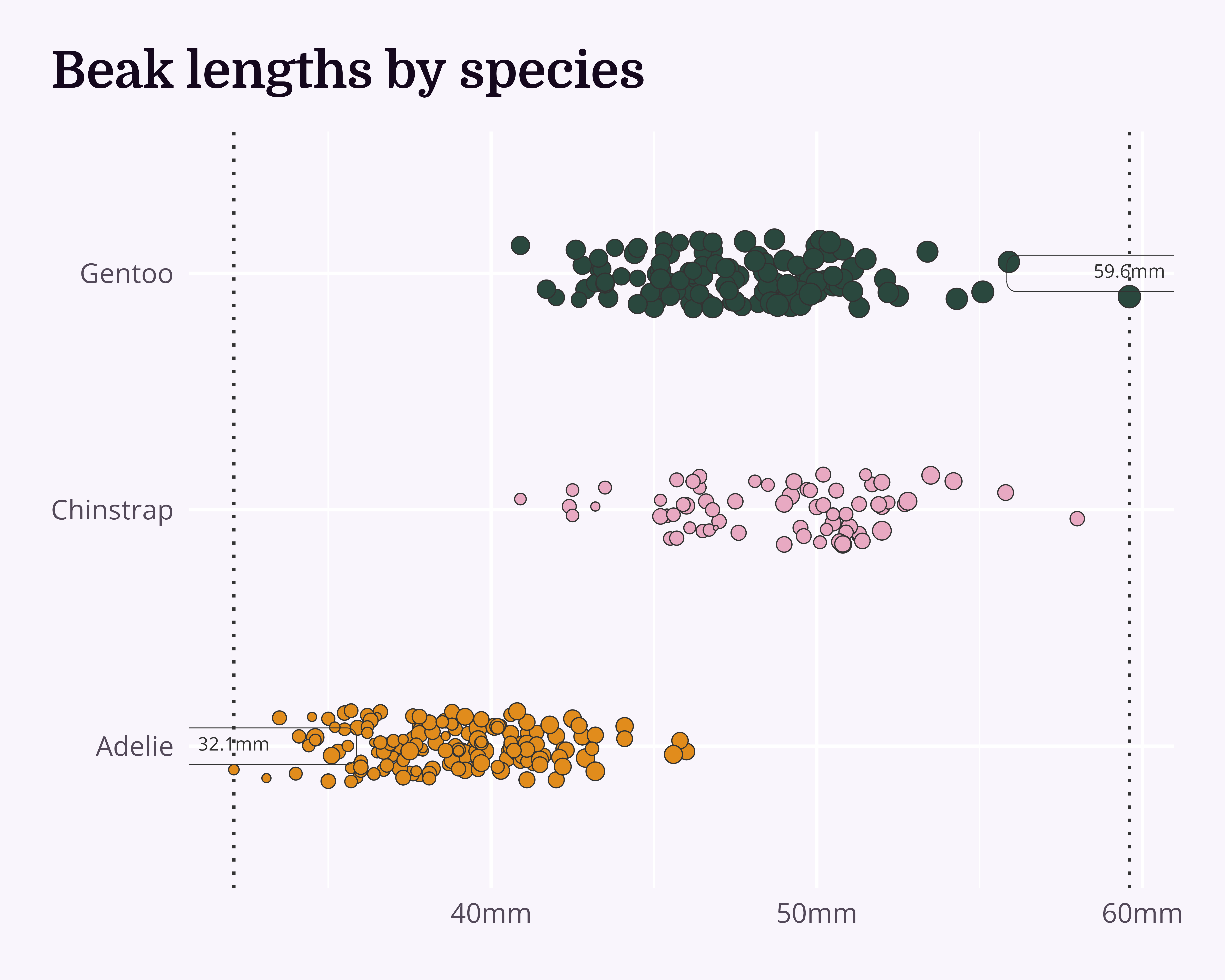
Annotations
Shift them out of the way of the data
penguin_df |>
  ggplot(aes(x = culmen_length_mm, y = species)) +
  geom_vline(
    data = beak_range_df,
    aes(xintercept = culmen_length_mm),
    linetype = 3,
    colour = "#333333"
  ) +
  geom_jitter(
    aes(
      x = culmen_length_mm,
      y = species,
      fill = species,
      size = body_mass_g
    ),
    shape = 21,
    width = 0,
    height = 0.15,
    colour = "#333333",
    stroke = 0.5
  ) +
  ggtext::geom_textbox(
    data = beak_range_df,
    aes(y = max(species), label = paste0(culmen_length_mm, "mm")),
    family = "Open Sans",
    halign = 0.5,
    colour = "#333333",
    fill = NA,
    nudge_y = 0.33
  ) +
  labs(title = "Beak lengths by species") +
  scale_fill_manual(values = penguin_colours) +
  scale_x_continuous(label = function(x) paste0(x, "mm")) +
  scale_y_discrete(labels = function(x) gsub("(.)( )(.*)", "\\1", x)) +
  theme_chester_penguins()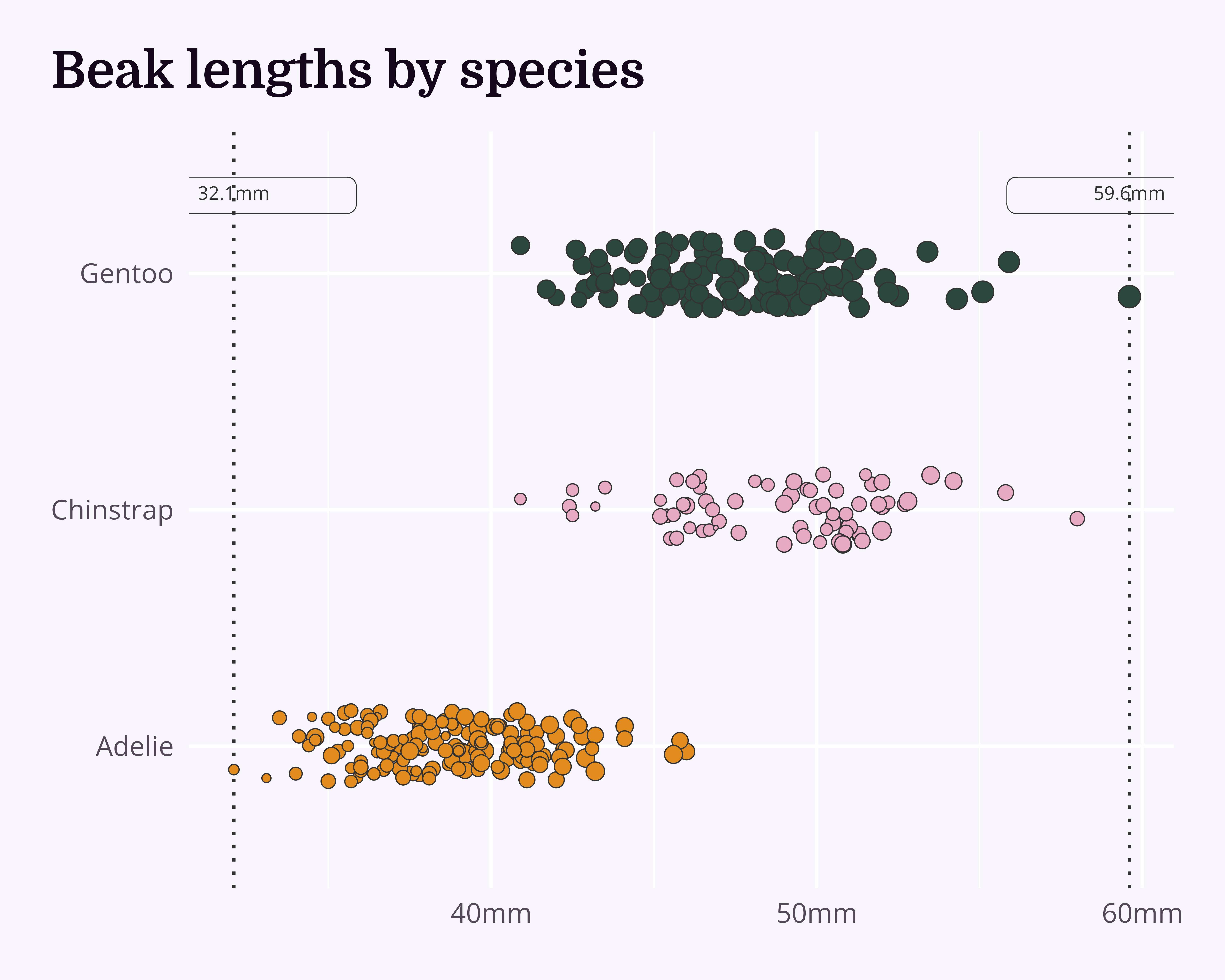
Annotations
Align them sensibly
penguin_df |>
  ggplot(aes(x = culmen_length_mm, y = species)) +
  geom_vline(
    data = beak_range_df,
    aes(xintercept = culmen_length_mm),
    linetype = 3,
    colour = "#333333"
  ) +
  geom_jitter(
    aes(
      x = culmen_length_mm,
      y = species,
      fill = species,
      size = body_mass_g
    ),
    shape = 21,
    width = 0,
    height = 0.15,
    colour = "#333333",
    stroke = 0.5
  ) +
  ggtext::geom_textbox(
    data = beak_range_df,
    aes(
      y = max(species),
      label = paste0(culmen_length_mm, "mm"),
      hjust = dplyr::case_when(
        culmen_length_mm == min(culmen_length_mm) ~ 0,
        TRUE ~ 1
      ),
      halign = dplyr::case_when(
        culmen_length_mm == min(culmen_length_mm) ~ 0,
        TRUE ~ 1
      )
    ),
    family = "Open Sans",
    colour = "#333333",
    fill = NA,
    nudge_y = 0.33
  ) +
  labs(title = "Beak lengths by species") +
  scale_fill_manual(values = penguin_colours) +
  scale_x_continuous(label = function(x) paste0(x, "mm")) +
  scale_y_discrete(labels = function(x) gsub("(.)( )(.*)", "\\1", x)) +
  theme_chester_penguins()
Annotations
Boldify
penguin_df |>
  ggplot(aes(x = culmen_length_mm, y = species)) +
  geom_vline(
    data = beak_range_df,
    aes(xintercept = culmen_length_mm),
    linetype = 3,
    colour = "#333333"
  ) +
  geom_jitter(
    aes(
      x = culmen_length_mm,
      y = species,
      fill = species,
      size = body_mass_g
    ),
    shape = 21,
    width = 0,
    height = 0.15,
    colour = "#333333",
    stroke = 0.5
  ) +
  ggtext::geom_textbox(
    data = beak_range_df,
    aes(
      y = max(species),
      label = paste0(culmen_length_mm, "mm"),
      hjust = dplyr::case_when(
        culmen_length_mm == min(culmen_length_mm) ~ 0,
        TRUE ~ 1
      ),
      halign = dplyr::case_when(
        culmen_length_mm == min(culmen_length_mm) ~ 0,
        TRUE ~ 1
      )
    ),
    family = "Open Sans",
    colour = "#333333",
    fontface = "bold",
    fill = NA,
    nudge_y = 0.33
  ) +
  labs(title = "Beak lengths by species") +
  scale_fill_manual(values = penguin_colours) +
  scale_x_continuous(label = function(x) paste0(x, "mm")) +
  scale_y_discrete(labels = function(x) gsub("(.)( )(.*)", "\\1", x)) +
  theme_chester_penguins()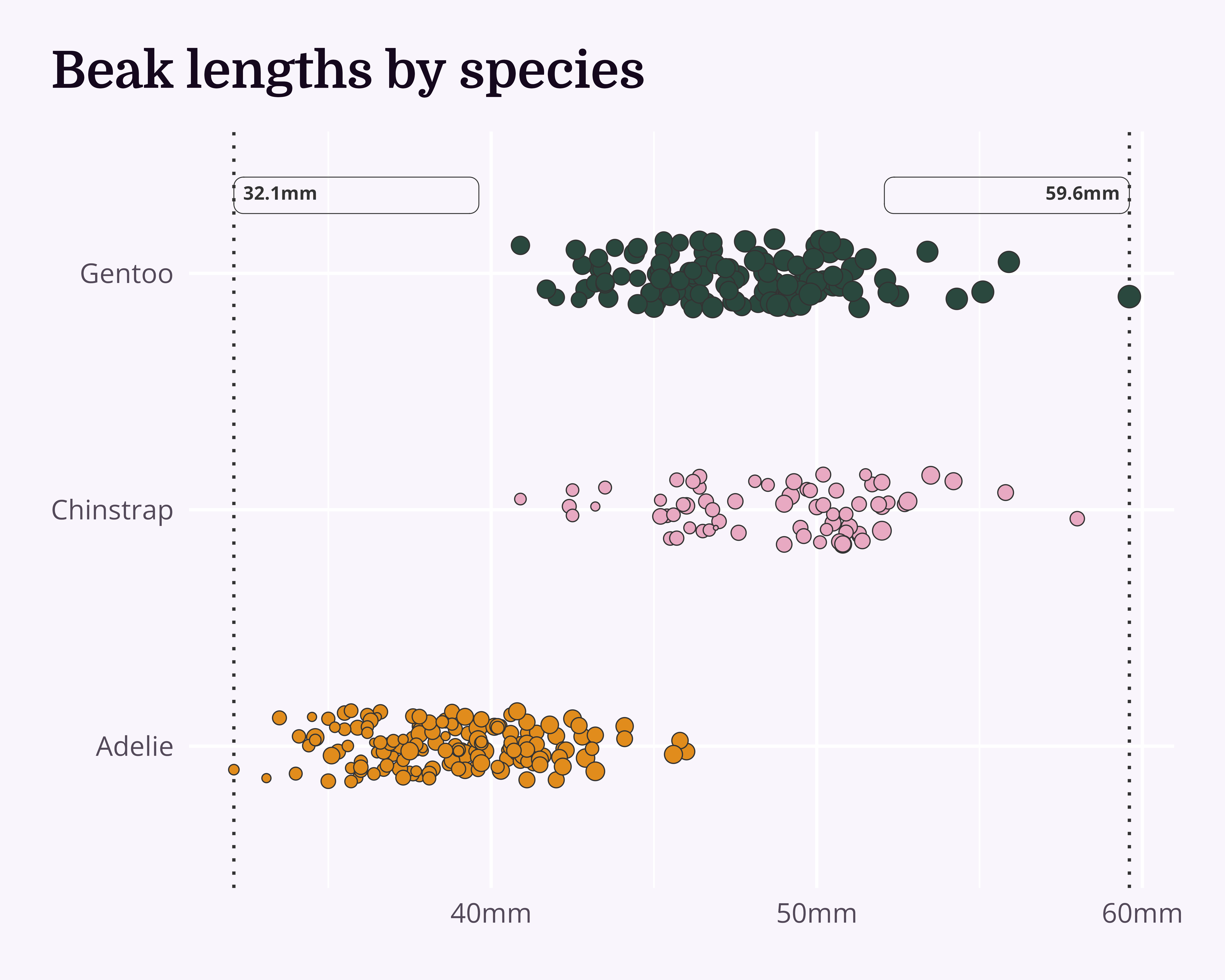
Annotations
Improve even more!
penguin_df |>
  ggplot(aes(x = culmen_length_mm, y = species)) +
  geom_vline(
    data = beak_range_df,
    aes(xintercept = culmen_length_mm),
    linetype = 3,
    colour = "#333333"
  ) +
  geom_jitter(
    aes(
      x = culmen_length_mm,
      y = species,
      fill = species,
      size = body_mass_g
    ),
    shape = 21,
    width = 0,
    height = 0.15,
    colour = "#333333",
    stroke = 0.5
  ) +
  ggtext::geom_textbox(
    data = beak_range_df,
    aes(
      y = max(species),
      label = dplyr::case_when(
        culmen_length_mm == min(culmen_length_mm) ~
          paste0("🞀 ", culmen_length_mm, "mm"),
        TRUE ~ paste0(culmen_length_mm, "mm", " 🞂")
      ),
      hjust = dplyr::case_when(
        culmen_length_mm == min(culmen_length_mm) ~ 0,
        TRUE ~ 1
      ),
      halign = dplyr::case_when(
        culmen_length_mm == min(culmen_length_mm) ~ 0,
        TRUE ~ 1
      )
    ),
    family = "Open Sans",
    colour = "#333333",
    fontface = "bold",
    fill = NA,
    box.padding = unit(0, "pt"),
    size = 5,
    box.colour = NA,
    nudge_y = 0.33
  ) +
  labs(title = "Beak lengths by species") +
  scale_fill_manual(values = penguin_colours) +
  scale_x_continuous(label = function(x) paste0(x, "mm")) +
  scale_y_discrete(labels = function(x) gsub("(.)( )(.*)", "\\1", x)) +
  theme_chester_penguins()
Annotations
And let’s add a bit more data…
beak_means_df <- penguin_df |>
  dplyr::group_by(species) |>
  dplyr::summarise(mean_length = mean(culmen_length_mm, na.rm = TRUE))

penguin_df |>
  ggplot(aes(x = culmen_length_mm, y = species)) +
  geom_vline(
    data = beak_range_df,
    aes(xintercept = culmen_length_mm),
    linetype = 3,
    colour = "#333333"
  ) +
  geom_segment(
    data = beak_means_df,
    aes(x = mean_length, xend = mean_length, y = -Inf, yend = species),
    linetype = 3
  ) +
  geom_jitter(
    aes(
      x = culmen_length_mm,
      y = species,
      fill = species,
      size = body_mass_g
    ),
    shape = 21,
    width = 0,
    height = 0.15,
    colour = "#333333",
    stroke = 0.5
  ) +
  ggtext::geom_textbox(
    data = beak_range_df,
    aes(
      y = max(species),
      label = dplyr::case_when(
        culmen_length_mm == min(culmen_length_mm) ~
          paste0("🞀 ", culmen_length_mm, "mm"),
        TRUE ~ paste0(culmen_length_mm, "mm", " 🞂")
      ),
      hjust = dplyr::case_when(
        culmen_length_mm == min(culmen_length_mm) ~ 0,
        TRUE ~ 1
      ),
      halign = dplyr::case_when(
        culmen_length_mm == min(culmen_length_mm) ~ 0,
        TRUE ~ 1
      )
    ),
    family = "Open Sans",
    colour = "#333333",
    fontface = "bold",
    fill = NA,
    box.padding = unit(0, "pt"),
    size = 5,
    box.colour = NA,
    nudge_y = 0.33
  ) +
  ggtext::geom_textbox(
    data = beak_means_df,
    aes(
      x = mean_length,
      y = species,
      label = paste0(
        species,
        " mean<br>**",
        janitor::round_half_up(mean_length),
        "mm**"
      )
    ),
    hjust = 0,
    nudge_y = -0.4,
    box.colour = NA,
    family = "Open Sans",
    colour = "#333333",
    fill = "#f9f5fc"
  ) +
  labs(title = "Beak lengths by species") +
  scale_fill_manual(values = penguin_colours) +
  scale_x_continuous(label = function(x) paste0(x, "mm")) +
  scale_y_discrete(labels = function(x) gsub("(.)( )(.*)", "\\1", x)) +
  theme_chester_penguins()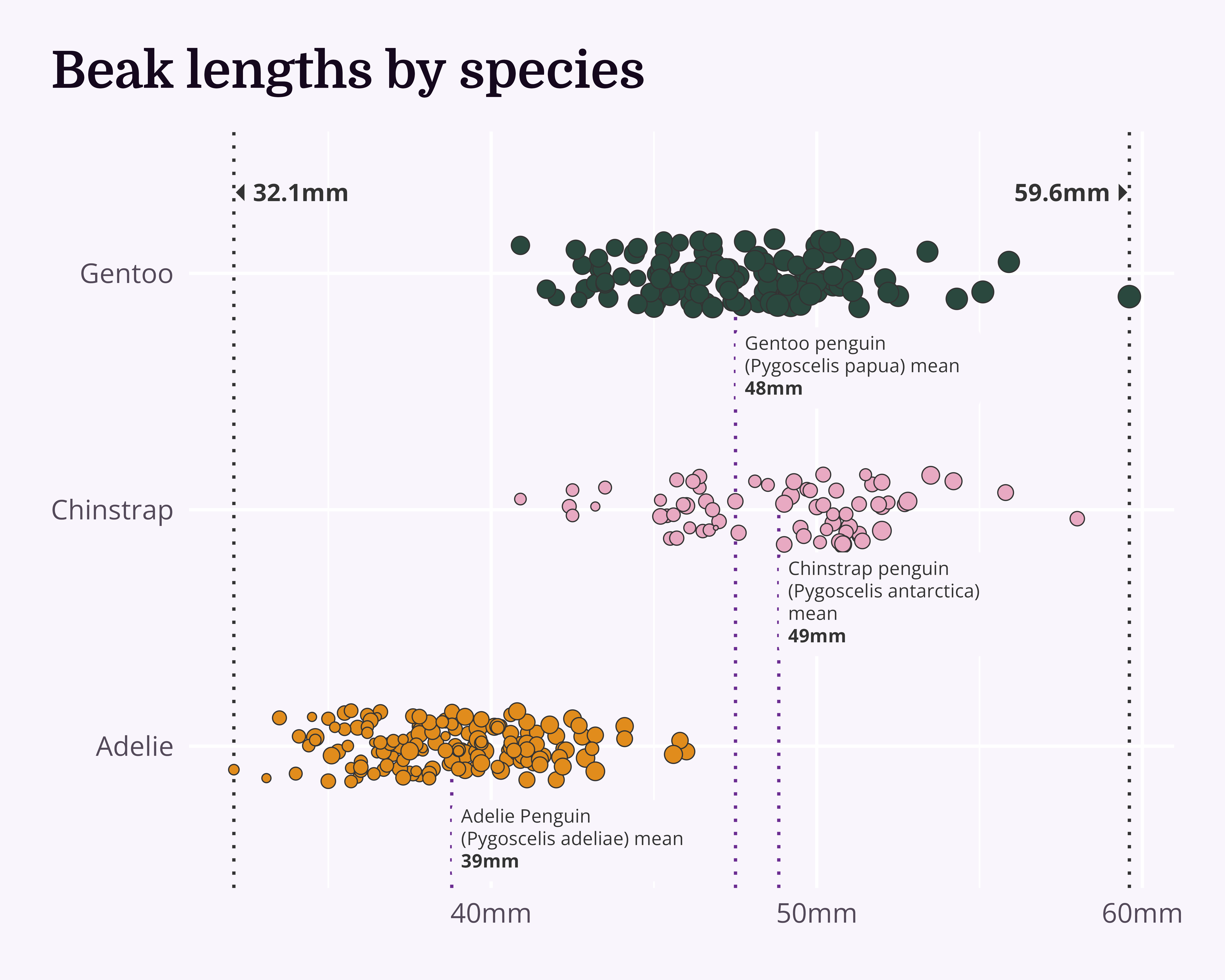
Annotations
And we can get rid of the y axis!
penguin_df |>
  ggplot(aes(x = culmen_length_mm, y = species)) +
  geom_vline(
    data = beak_range_df,
    aes(xintercept = culmen_length_mm),
    linetype = 3,
    colour = "#333333"
  ) +
  geom_segment(
    data = beak_means_df,
    aes(x = mean_length, xend = mean_length, y = -Inf, yend = species),
    linetype = 3
  ) +
  geom_jitter(
    aes(
      x = culmen_length_mm,
      y = species,
      fill = species,
      size = body_mass_g
    ),
    shape = 21,
    width = 0,
    height = 0.15,
    colour = "#333333",
    stroke = 0.5
  ) +
  ggtext::geom_textbox(
    data = beak_range_df,
    aes(
      y = max(species),
      label = dplyr::case_when(
        culmen_length_mm == min(culmen_length_mm) ~
          paste0("🞀 ", culmen_length_mm, "mm"),
        TRUE ~ paste0(culmen_length_mm, "mm", " 🞂")
      ),
      hjust = dplyr::case_when(
        culmen_length_mm == min(culmen_length_mm) ~ 0,
        TRUE ~ 1
      ),
      halign = dplyr::case_when(
        culmen_length_mm == min(culmen_length_mm) ~ 0,
        TRUE ~ 1
      )
    ),
    family = "Open Sans",
    colour = "#333333",
    fontface = "bold",
    fill = NA,
    box.padding = unit(0, "pt"),
    size = 5,
    box.colour = NA,
    nudge_y = 0.33
  ) +
  ggtext::geom_textbox(
    data = beak_means_df,
    aes(
      x = mean_length,
      y = species,
      label = paste0(
        species,
        " mean<br>**",
        janitor::round_half_up(mean_length),
        "mm**"
      )
    ),
    hjust = 0,
    nudge_y = -0.4,
    box.colour = NA,
    family = "Open Sans",
    colour = "#333333",
    fill = "#f9f5fc"
  ) +
  labs(title = "Beak lengths by species") +
  scale_fill_manual(values = penguin_colours) +
  scale_x_continuous(label = function(x) paste0(x, "mm")) +
  scale_y_discrete(labels = function(x) gsub("(.)( )(.*)", "\\1", x)) +
  theme_chester_penguins() +
  theme(axis.text.y = element_blank())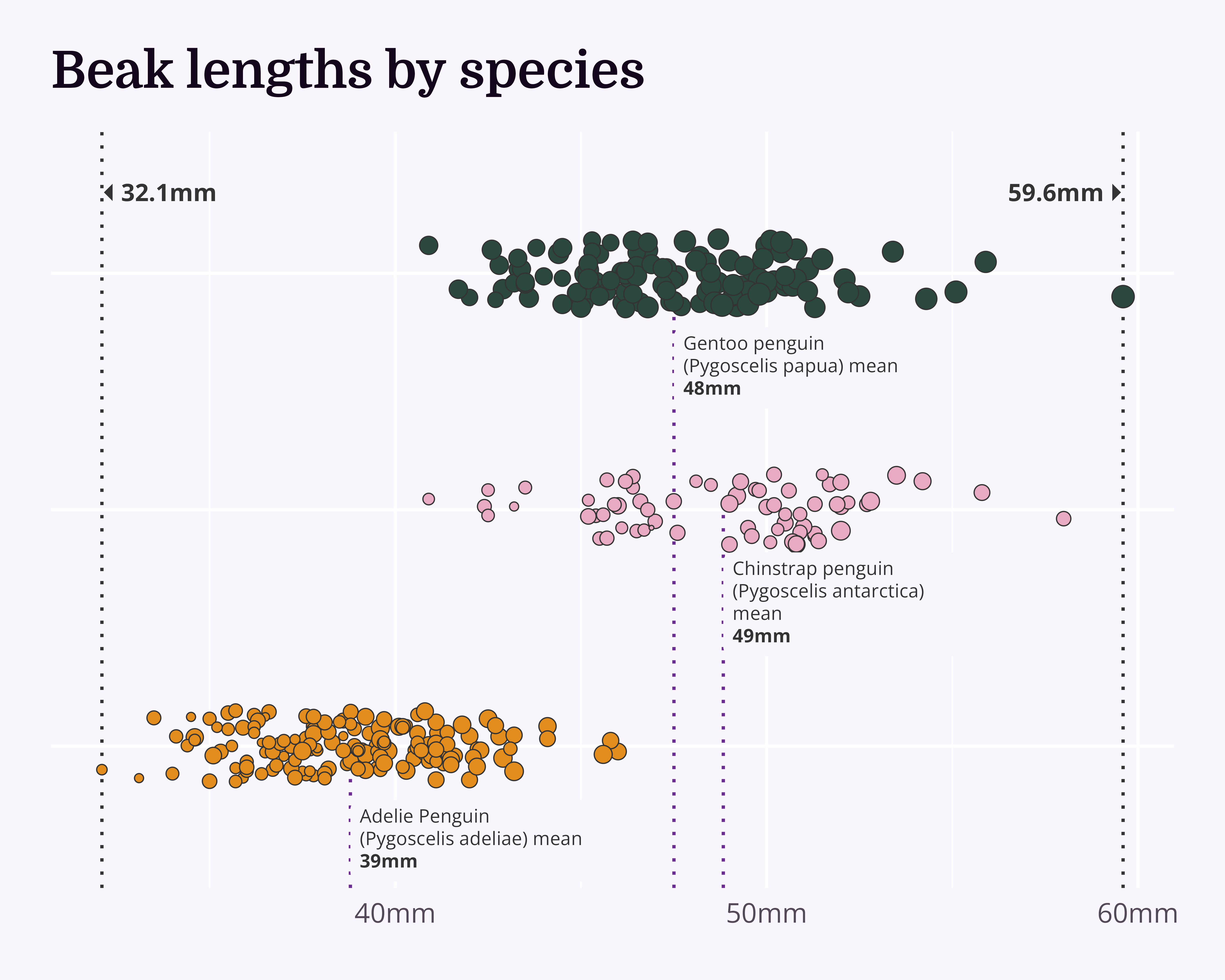
We’ve already come quite far!
Happy datavizing!

cararthompson.com/talkshello@cararthompson.comcararthompson.com/newsletter